MODEL EVALUATION & OPTIMIZATION
7 basic classifiers reveal their prediction confidence math
Classification models don’t just tell you what they think the answer is — they also tell you how sure they are about that answer. This certainty is shown as a probability score. A high score means the model is very confident, while a low score means it’s uncertain about its prediction.
Every classification model calculates these probability scores differently. Simple models and complex ones each have their own specific methods to determine the likelihood of each possible outcome.
We’re going to explore seven basic classification models and visually break down how each one figures out its probability scores. No need for a crystal ball — we’ll make these probability calculations crystal clear!

Definition
Predicted probability (or “class probability”) is a number from 0 to 1 (or 0% to 100%) that shows how confident a model is about its answer. If the number is 1, the model is completely sure about its answer. If it’s 0.5, the model is basically guessing — it’s like flipping a coin.
Components of a Probability Score
When a model has to choose between two classes (called binary classification), three main rules apply:
- The predicted probability must be between 0 and 1
- The chances of both options happening must add up to 1
- A higher probability means the model is more sure about its choice

For binary classification, when we talk about predicted probability, we usually mean the probability of the positive class. A higher probability means the model thinks the positive class is more likely, while a lower probability means it thinks the negative class is more likely.
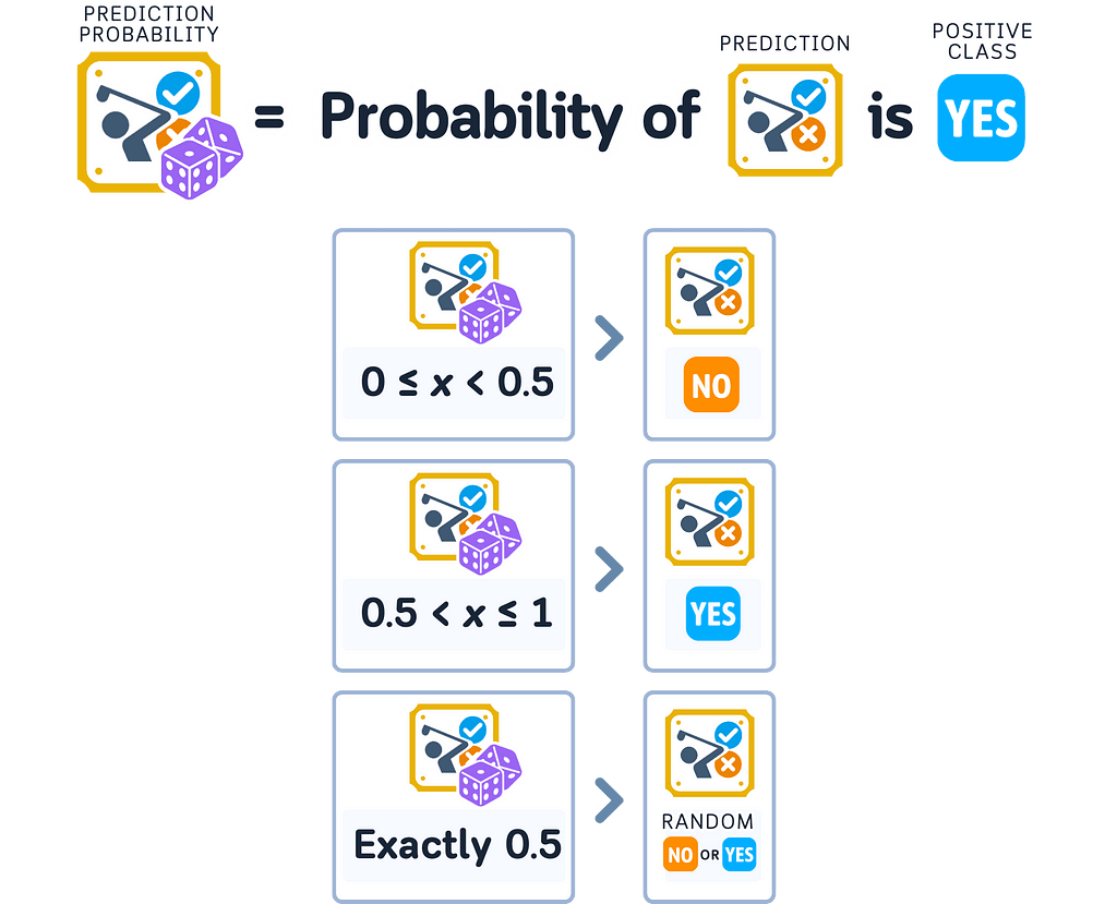
To make sure these rules are followed, models use mathematical functions to convert their calculations into proper probabilities. Each type of model might use different functions, which affects how they express their confidence levels.
Prediction vs. Probability
In classification, a model picks the class it thinks will most likely happen — the one with the highest probability score. But two different models might pick the same class while being more or less confident about it. Their predicted probability scores tell us how sure each model is, even when they make the same choice.
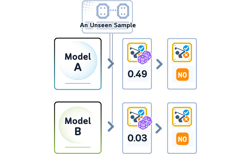
These different probability scores tell us something important: even when models pick the same class, they might understand the data differently.
One model might be very sure about its choice, while another might be less confident — even though they made the same prediction.
📊 Dataset Used
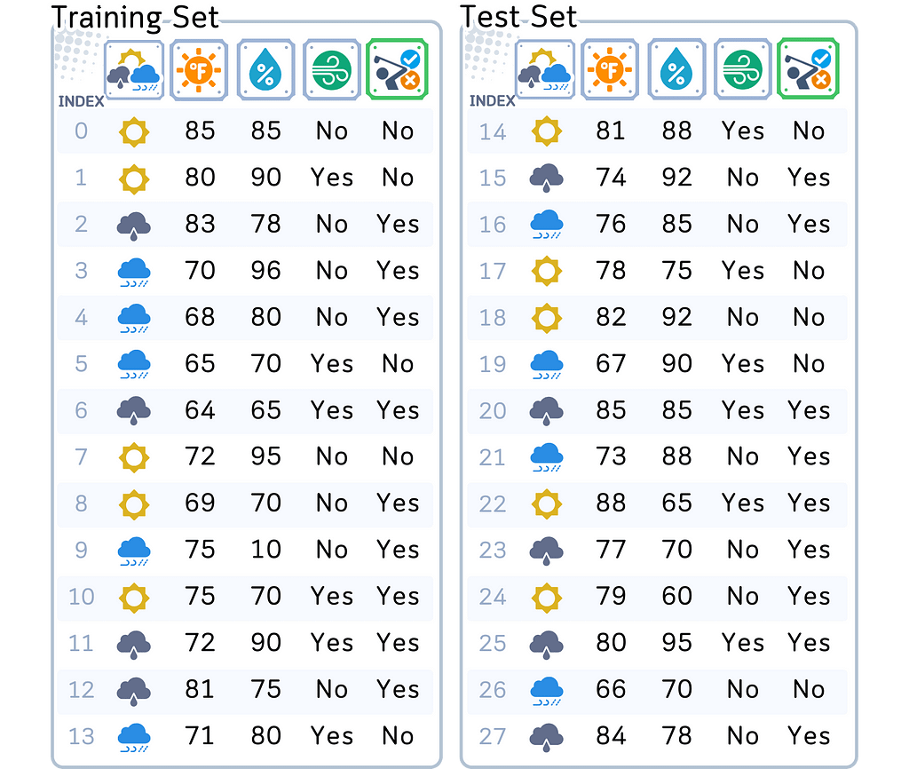
To understand how predicted probability is calculated, we’ll continue with the same dataset used in my previous articles on Classification Algorithms. Our goal remains: predicting if someone will play golf based on the weather.
import pandas as pd
import numpy as np
from sklearn.metrics import accuracy_score
from sklearn.model_selection import train_test_split

# Create and prepare dataset
dataset_dict = {
    'Outlook': ['sunny', 'sunny', 'overcast', 'rainy', 'rainy', 'rainy', 'overcast',
                'sunny', 'sunny', 'rainy', 'sunny', 'overcast', 'overcast', 'rainy',
                'sunny', 'overcast', 'rainy', 'sunny', 'sunny', 'rainy', 'overcast',
                'rainy', 'sunny', 'overcast', 'sunny', 'overcast', 'rainy', 'overcast'],
    'Temperature': [85.0, 80.0, 83.0, 70.0, 68.0, 65.0, 64.0, 72.0, 69.0, 75.0, 75.0,
                   72.0, 81.0, 71.0, 81.0, 74.0, 76.0, 78.0, 82.0, 67.0, 85.0, 73.0,
                   88.0, 77.0, 79.0, 80.0, 66.0, 84.0],
    'Humidity': [85.0, 90.0, 78.0, 96.0, 80.0, 70.0, 65.0, 95.0, 70.0, 80.0, 70.0,
                 90.0, 75.0, 80.0, 88.0, 92.0, 85.0, 75.0, 92.0, 90.0, 85.0, 88.0,
                 65.0, 70.0, 60.0, 95.0, 70.0, 78.0],
    'Wind': [False, True, False, False, False, True, True, False, False, False, True,
             True, False, True, True, False, False, True, False, True, True, False,
             True, False, False, True, False, False],
    'Play': ['No', 'No', 'Yes', 'Yes', 'Yes', 'No', 'Yes', 'No', 'Yes', 'Yes', 'Yes',
             'Yes', 'Yes', 'No', 'No', 'Yes', 'Yes', 'No', 'No', 'No', 'Yes', 'Yes',
             'Yes', 'Yes', 'Yes', 'Yes', 'No', 'Yes']
}

# Prepare data
df = pd.DataFrame(dataset_dict)
As some algorithms might need standardized values, we will also do standard scaling to the numerical features and one-hot encoding to the categorical features, including the target feature:

from sklearn.preprocessing import StandardScaler
df = pd.get_dummies(df, columns=['Outlook'], prefix='', prefix_sep='', dtype=int)
df['Wind'] = df['Wind'].astype(int)
df['Play'] = (df['Play'] == 'Yes').astype(int)

# Rearrange columns
column_order = ['sunny', 'overcast', 'rainy', 'Temperature', 'Humidity', 'Wind', 'Play']
df = df[column_order]

# Prepare features and target
X,y = df.drop('Play', axis=1), df['Play']
X_train, X_test, y_train, y_test = train_test_split(X, y, train_size=0.5, shuffle=False)

# Scale numerical features
scaler = StandardScaler()
X_train[['Temperature', 'Humidity']] = scaler.fit_transform(X_train[['Temperature', 'Humidity']])
X_test[['Temperature', 'Humidity']] = scaler.transform(X_test[['Temperature', 'Humidity']])
Now, let’s see how each of the following 7 classification algorithms calculates these probabilities:

Dummy Classifier Probabilities
Dummy Classifier Explained: A Visual Guide with Code Examples for Beginners
A Dummy Classifier is a prediction model that doesn’t learn patterns from data. Instead, it follows basic rules like: picking the most common outcome, making random predictions based on how often each outcome appeared in training, always picking one answer, or randomly choosing between options with equal chance. The Dummy Classifier ignores all input features and just follows these rules.
When this model finishes training, all it remembers is a few numbers showing either how often each outcome happened or the constant values it was told to use. It doesn’t learn anything about how features relate to outcomes.

For calculating predicted probability in binary classification, the Dummy Classifier uses the most basic approach possible. Since it only remembered how often each outcome appeared in the training data, it uses these same numbers as probability scores for every prediction — either 0 or 1.

These probability scores stay exactly the same for all new data, because the model doesn’t look at or react to any features of the new data it’s trying to predict.
from sklearn.dummy import DummyClassifier
import pandas as pd
import numpy as np

# Train the model
dummy_clf = DummyClassifier(strategy='stratified', random_state=42)
dummy_clf.fit(X_train, y_train)

# Print the "model" - which is just the class probabilities
print("THE MODEL:")
print(f"Probability of not playing (class 0): {dummy_clf.class_prior_[0]:.3f}")
print(f"Probability of playing (class 1): {dummy_clf.class_prior_[1]:.3f}")
print("nNOTE: These probabilities are used for ALL predictions, regardless of input features!")

# Make predictions and get probabilities
y_pred = dummy_clf.predict(X_test)
y_prob = dummy_clf.predict_proba(X_test)

# Create results dataframe
results_df = pd.DataFrame({
    'True Label': y_test,
    'Prediction': y_pred,
    'Probability of Play': y_prob[:, 1]
})

print("nPrediction Results:")
print(results_df)
print(f"Accuracy: {accuracy_score(y_test, y_pred)}")
k-Nearest Neighbors (KNN) Probabilities
K Nearest Neighbor Classifier, Explained: A Visual Guide with Code Examples for Beginners
K-Nearest Neighbors (kNN) is a prediction model that takes a different approach — instead of learning rules, it keeps all training examples in memory. When it needs to make a prediction about new data, it measures how similar this data is to every stored example, finds the k most similar ones (where k is a number we choose), and makes its decision based on those neighbors.
When this model finishes training, all it has stored is the complete training dataset, the value of k we chose, and a method for measuring how similar two data points are (by default using Euclidean distance).
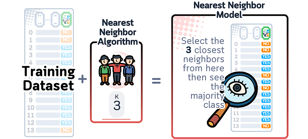
For calculating predicted probability, kNN looks at those k most similar examples and counts how many belong to each class. The probability score is simply the number of neighbors belonging to a class divided by k.
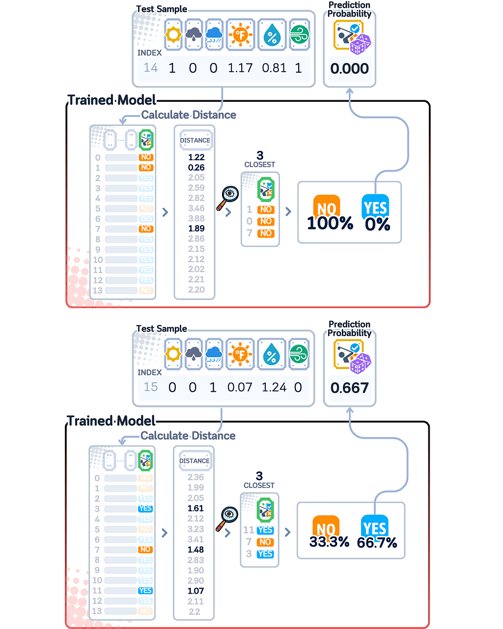
Since kNN calculates probability scores by division, it can only give certain specific values based on k (say, for k=5, the only possible probability scores are 0/5 (0%), 1/5 (20%), 2/5 (40%), 3/5 (60%), 4/5 (80%), and 5/5 (100%)). This means kNN can’t give as many different confidence levels as other models.
from sklearn.neighbors import KNeighborsClassifier
import pandas as pd
import numpy as np

# Train the model
k = 3  # number of neighbors
knn = KNeighborsClassifier(n_neighbors=k)
knn.fit(X_train, y_train)

# Print the "model"
print("THE MODEL:")
print(f"Number of neighbors (k): {k}")
print(f"Training data points stored: {len(X_train)}")

# Make predictions and get probabilities
y_pred = knn.predict(X_test)
y_prob = knn.predict_proba(X_test)

# Create results dataframe
results_df = pd.DataFrame({
   'True Label': y_test,
   'Prediction': y_pred,
   'Probability of Play': y_prob[:, 1]
})

print("nPrediction Results:")
print(results_df)
print(f"Accuracy: {accuracy_score(y_test, y_pred)}")
Naive Bayes Probabilities
Bernoulli Naive Bayes, Explained: A Visual Guide with Code Examples for Beginners
Naive Bayes is a prediction model that uses probability math with a “naive” rule: it assumes each feature affects the outcome independently. There are different types of Naive Bayes: Gaussian Naive Bayes works with continuous values, while Bernoulli Naive Bayes works with binary features. As our dataset has many 0–1 features, we’ll focus on the Bernoulli one here.
When this model finishes training, it remembers probability values: one value for how often the positive class occurs, and for each feature, values showing how likely different feature values appear when we have a positive outcome.
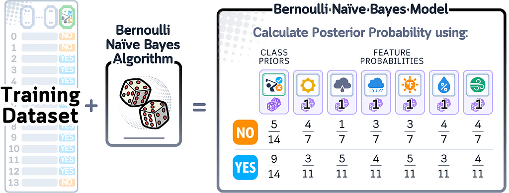
For calculating predicted probability, Naive Bayes multiplies several probabilities together: the chance of each class occurring, and the chance of seeing each feature value within that class. These multiplied probabilities are then normalized so they sum to 1, giving us the final probability scores.
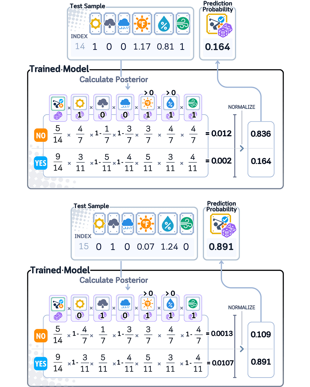
Since Naive Bayes uses probability math, its probability scores naturally fall between 0 and 1. However, when certain features strongly point to one class over another, the model can give probability scores very close to 0 or 1, showing it’s very confident about its prediction.
from sklearn.naive_bayes import BernoulliNB
import pandas as pd

# Train the model
nb = BernoulliNB()
nb.fit(X_train, y_train)

# Print the "model"
print("THE MODEL:")
df = pd.DataFrame(
   nb.feature_log_prob_.T,
   columns=['Log Prob (No Play)', 'Log Prob (Play)'],
   index=['sunny', 'overcast', 'rainy', 'Temperature', 'Humidity', 'Wind']
)
df = df.round(3)
print("nFeature Log-Probabilities:")
print(df)

print("nClass Priors:")
priors = pd.Series(nb.class_log_prior_, index=['No Play', 'Play']).round(3)
print(priors)

# Make predictions and get probabilities
y_pred = nb.predict(X_test)
y_prob = nb.predict_proba(X_test)

# Create results dataframe
results_df = pd.DataFrame({
   'True Label': y_test,
   'Prediction': y_pred,
   'Probability of Play': y_prob[:, 1]
})

print("nPrediction Results:")
print(results_df)
print(f"Accuracy: {accuracy_score(y_test, y_pred)}")
Decision Tree Probabilities
Decision Tree Classifier, Explained: A Visual Guide with Code Examples for Beginners
A Decision Tree Classifier works by creating a series of yes/no questions about the input data. It builds these questions one at a time, always choosing the most useful question that best separates the data into groups. It keeps asking questions until it reaches a final answer at the end of a branch.
When this model finishes training, it has created a tree where each point represents a question about the data. Each branch shows which way to go based on the answer, and at the end of each branch is information about how often each class appeared in the training data.
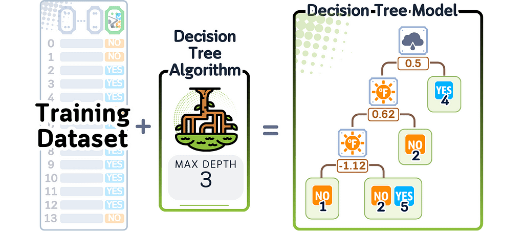
For calculating predicted probability, the Decision Tree follows all its questions for new data until it reaches the end of a branch. The probability score is based on how many training examples of each class ended up at that same branch during training.
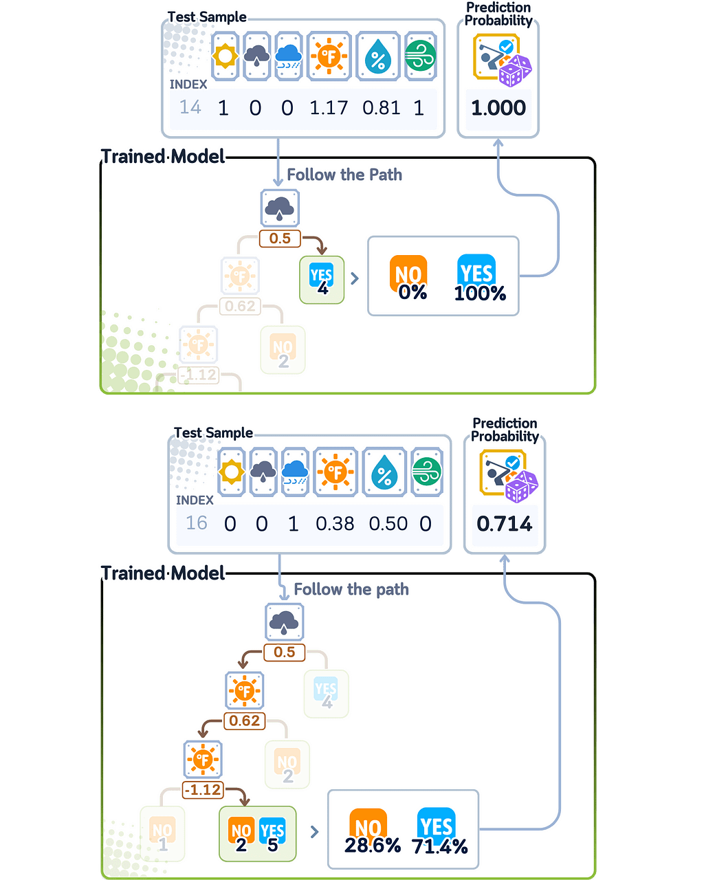
Since Decision Tree probability scores come from counting training examples at each branch endpoint, they can only be certain values that were seen during training. This means the model can only give probability scores that match the patterns it found while learning, which limits how precise its confidence levels can be.
from sklearn.tree import DecisionTreeClassifier, plot_tree
import pandas as pd
import matplotlib.pyplot as plt

# Train the model
dt = DecisionTreeClassifier(random_state=42, max_depth=3)  # limiting depth for visibility
dt.fit(X_train, y_train)

# Print the "model" - visualize the decision tree
print("THE MODEL (DECISION TREE STRUCTURE):")
plt.figure(figsize=(20,10))
plot_tree(dt, feature_names=['sunny', 'overcast', 'rainy', 'Temperature',
                           'Humidity', 'Wind'],
         class_names=['No Play', 'Play'],
         filled=True, rounded=True, fontsize=10)
plt.show()

# Make predictions and get probabilities
y_pred = dt.predict(X_test)
y_prob = dt.predict_proba(X_test)

# Create results dataframe
results_df = pd.DataFrame({
   'True Label': y_test,
   'Prediction': y_pred,
   'Probability of Play': y_prob[:, 1]
})

print("nPrediction Results:")
print(results_df)
print(f"Accuracy: {accuracy_score(y_test, y_pred)}")
Logistic Regression Probabilities
Logistic Regression, Explained: A Visual Guide with Code Examples for Beginners
A Logistic Regression model, despite its name, predicts between two classes using a mathematical equation. For each feature in the input data, it learns how important that feature is by giving it a number (weight). It also learns one extra number (bias) that helps make better predictions. To turn these numbers into a predicted probability, it uses the sigmoid function that keeps the final answer between 0 and 1.
When this model finishes training, all it remembers is these weights — one number for each feature, plus the bias number. These numbers are all it needs to make predictions.
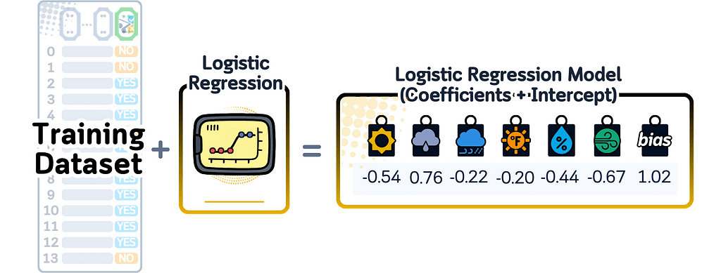
For calculating predicted probability in binary classification, Logistic Regression first multiplies each feature value by its weight and adds them all together, plus the bias. This sum could be any number, so the model uses the sigmoid function to convert it into a probability between 0 and 1.
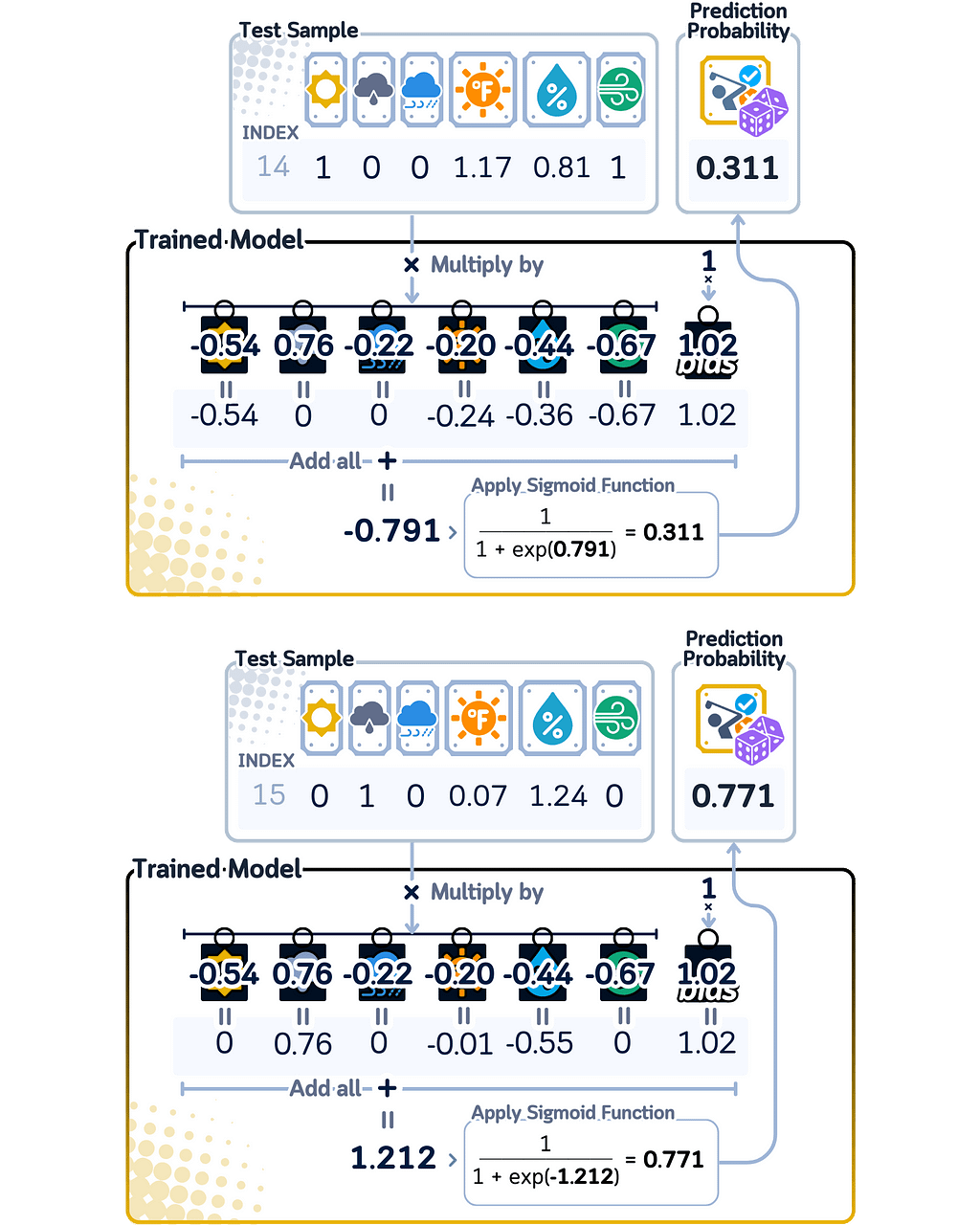
Unlike other models that can only give certain specific probability scores, Logistic Regression can give any probability between 0 and 1. The further the input data is from the point where the model switches from one class to another (the decision boundary), the closer the probability gets to either 0 or 1. Data points near this switching point get probabilities closer to 0.5, showing the model is less confident about these predictions.
from sklearn.linear_model import LogisticRegression
import pandas as pd

# Train the model
lr = LogisticRegression(random_state=42)
lr.fit(X_train, y_train)

# Print the "model"
print("THE MODEL:")
model_df = pd.DataFrame({
   'Feature': ['sunny', 'overcast', 'rainy', 'Temperature', 'Humidity', 'Wind'],
   'Coefficient': lr.coef_[0]
})
model_df['Coefficient'] = model_df['Coefficient'].round(3)
print("Coefficients (weights):")
print(model_df)

print(f"nIntercept (bias): {lr.intercept_[0]:.3f}")
print("nPrediction = sigmoid(intercept + sum(coefficient * feature_value))")

# Make predictions and get probabilities
y_pred = lr.predict(X_test)
y_prob = lr.predict_proba(X_test)

# Create results dataframe
results_df = pd.DataFrame({
   'True Label': y_test,
   'Prediction': y_pred,
   'Probability of Play': y_prob[:, 1]
})

print("nPrediction Results:")
print(results_df)
print(f"Accuracy: {accuracy_score(y_test, y_pred)}")
Support Vector Machine (SVM) Probabilities
Support Vector Classifier, Explained: A Visual Guide with Mini 2D Dataset
A Support Vector Machine (SVM) Classifier works by finding the best boundary line (or surface) that separates different classes. It focuses on the points closest to this boundary (called support vectors). While the basic SVM finds straight boundary lines, it can also create curved boundaries using mathematical functions called kernels.
When this model finishes training, it remembers three things: the important points near the boundary (support vectors), how much each point matters (weights), and any settings for curved boundaries (kernel parameters). Together, these define where and how the boundary separates the classes.
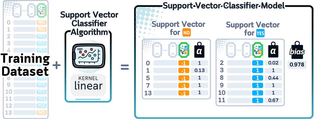
For calculating predicted probability in binary classification, SVM needs an extra step because it wasn’t designed to give probability scores. It uses a method called Platt Scaling, which adds a Logistic Regression layer to convert distances from the boundary into probabilities. These distances go through the sigmoid function to get final probability scores.
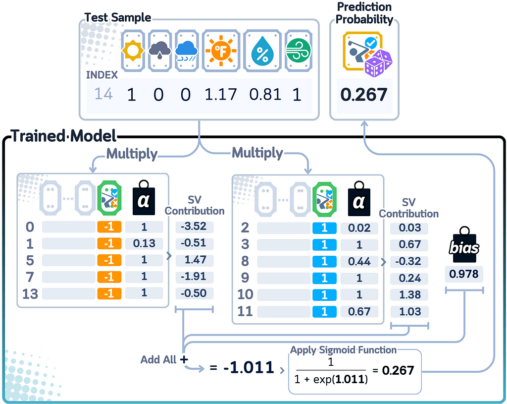
Since SVM calculates probabilities this indirect way, the scores show how far points are from the boundary rather than true confidence levels. Points far from the boundary get probability scores closer to 0 or 1, while points near the boundary get scores closer to 0.5. This means the probability scores are more about location relative to the boundary than the model’s actual confidence in its predictions.
from sklearn.svm import SVC
import pandas as pd
import numpy as np

# Train the model
svm = SVC(kernel='rbf', probability=True, random_state=42)
svm.fit(X_train, y_train)

# Print the "model"
print("THE MODEL:")
print(f"Kernel: {svm.kernel}")
print(f"Number of support vectors: {svm.n_support_}")
print("nSupport Vectors (showing first 5 rows):")

# Create dataframe of support vectors
sv_df = pd.DataFrame(
   svm.support_vectors_,
   columns=['sunny', 'overcast', 'rainy', 'Temperature', 'Humidity', 'Wind']
)
print(sv_df.head().round(3))

# Show which classes these support vectors belong to
print("nSupport vector classes:")
for i, count in enumerate(svm.n_support_):
   print(f"Class {i}: {count} support vectors")

# Make predictions and get probabilities
y_pred = svm.predict(X_test)
y_prob = svm.predict_proba(X_test)

# Create results dataframe
results_df = pd.DataFrame({
   'True Label': y_test,
   'Prediction': y_pred,
   'Probability of Play': y_prob[:, 1]
})

print("nPrediction Results:")
print(results_df)
print(f"Accuracy: {accuracy_score(y_test, y_pred)}")
Multilayer Perceptron Probabilities
Multilayer Perceptron, Explained: A Visual Guide with Mini 2D Dataset
A Multi-Layer Perceptron (MLP) Classifier is a type of neural network that processes data through several layers of connected nodes (neurons). Each neuron calculates a weighted total of its inputs, transforms this number using a function (like ReLU), and sends the result to the next layer. For binary classification, the last layer uses the sigmoid function to give an output between 0 and 1.
When this model finishes training, it remembers two main things: the connection strengths (weights and biases) between neurons in neighboring layers, and how the network is structured (how many layers and neurons are in each layer).
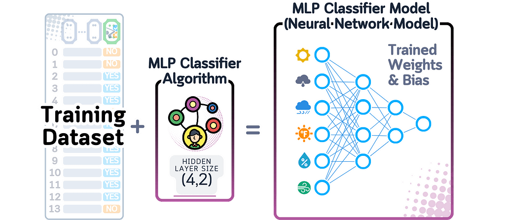
For calculating predicted probability in binary classification, the MLP moves data through its layers, with each layer creating more complex combinations of information from the previous layer. The final layer produces a number that the sigmoid function converts into a probability between 0 and 1.
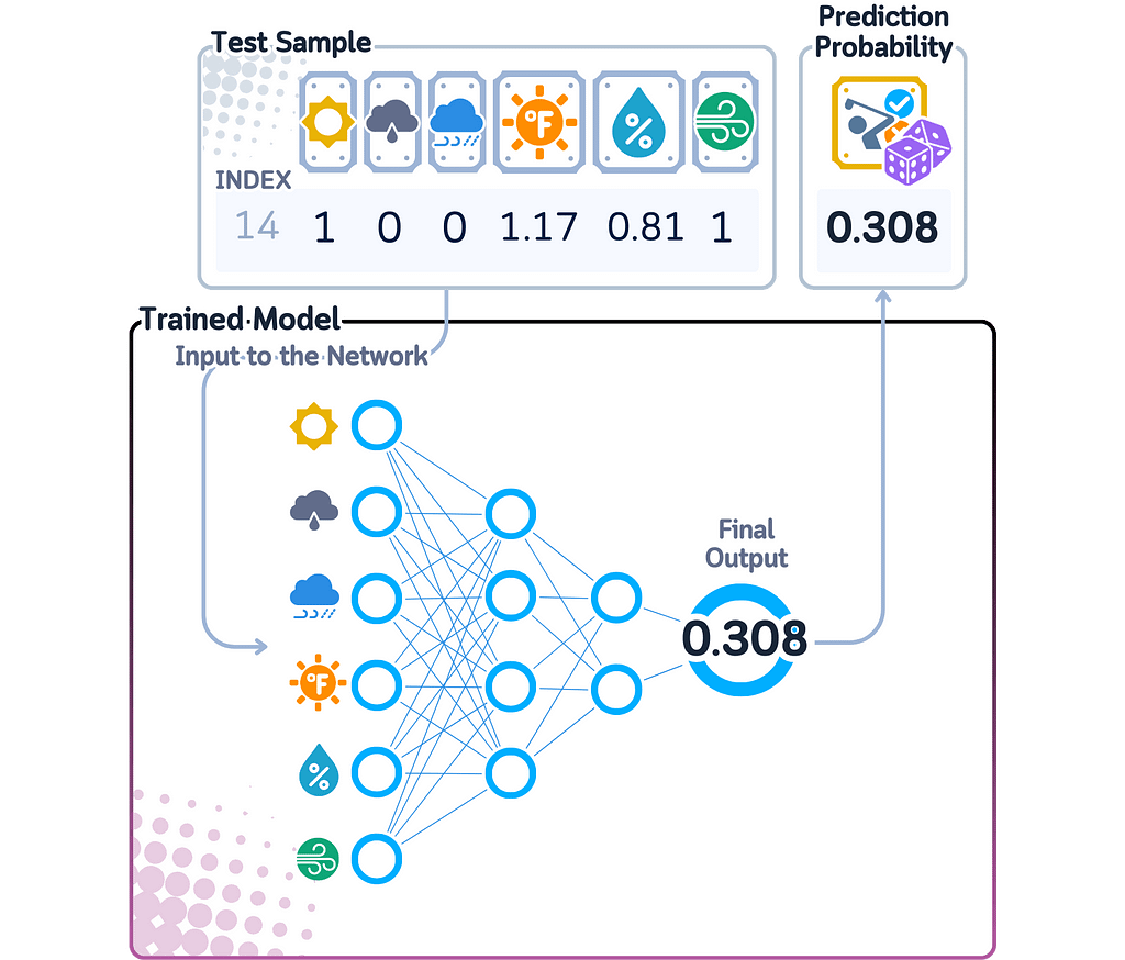
The MLP can find more complex patterns in data than many other models because it combines features in advanced ways. The final probability score shows how confident the network is — scores close to 0 or 1 mean the network is very confident about its prediction, while scores near 0.5 indicate it’s uncertain.
from sklearn.neural_network import MLPClassifier
import pandas as pd
import numpy as np

# Train the model with a simple architecture
mlp = MLPClassifier(hidden_layer_sizes=(4,2), random_state=42)
mlp.fit(X_train, y_train)

# Print the "model"
print("THE MODEL:")
print("Network Architecture:")
print(f"Input Layer: {mlp.n_features_in_} neurons (features)")
for i, layer_size in enumerate(mlp.hidden_layer_sizes):
   print(f"Hidden Layer {i+1}: {layer_size} neurons")
print(f"Output Layer: {mlp.n_outputs_} neurons (classes)")

# Show weights for first hidden layer
print("nWeights from Input to First Hidden Layer:")
weights_df = pd.DataFrame(
   mlp.coefs_[0],
   columns=[f'Hidden_{i+1}' for i in range(mlp.hidden_layer_sizes[0])],
   index=['sunny', 'overcast', 'rainy', 'Temperature', 'Humidity', 'Wind']
)
print(weights_df.round(3))

print("nNote: Additional weights and biases exist between subsequent layers")

# Make predictions and get probabilities
y_pred = mlp.predict(X_test)
y_prob = mlp.predict_proba(X_test)

# Create results dataframe
results_df = pd.DataFrame({
   'True Label': y_test,
   'Prediction': y_pred,
   'Probability of Play': y_prob[:, 1]
})

print("nPrediction Results:")
print(results_df)
print(f"Accuracy: {accuracy_score(y_test, y_pred)}")
Model Comparison
To summarize, here’s how each classifier calculates predicted probabilities:
- Dummy Classifier: Uses the same probability scores for all predictions, based only on how often each class appeared in training. Ignores all input features.
- K-Nearest Neighbors: The probability score is the fraction of similar neighbors belonging to each class. Can only give specific fractions based on k (like 3/5 or 7/10).
- Naive Bayes: Multiplies together the initial class probability and probabilities of seeing each feature value, then adjusts the results to add up to 1. Probability scores show how likely features are to appear in each class.
- Decision Tree: Gives probability scores based on how often each class appeared in the final branches. Can only use probability values that it saw during training.
- Logistic Regression: Uses the sigmoid function to convert weighted feature combinations into probability scores. Can give any probability between 0 and 1, changing smoothly based on distance from the decision boundary.
- Support Vector Machine: Needs an extra step (Platt Scaling) to create probability scores, using the sigmoid function to convert distances from the boundary. These distances determine how confident the model is.
- Multi-Layer Perceptron: Processes data through multiple layers of transformations, ending with the sigmoid function. Creates probability scores from complex feature combinations, giving any value between 0 and 1.
Final Remark
Looking at how each model calculates its predicted probability shows us something important: each model has its own way of showing how confident it is. Some models like the Dummy Classifier and Decision Tree can only use certain probability scores based on their training data. Others like Logistic Regression and Neural Networks can give any probability between 0 and 1, letting them be more precise about their uncertainty.
Here’s what’s interesting: even though all these models give us numbers between 0 and 1, these numbers mean different things for each model. Some get their scores by simple counting, others by measuring distance from a boundary, and some through complex calculations with features. This means a 70% probability from one model tells us something completely different than a 70% from another model.
When picking a model to use, look beyond just accuracy. Think about whether the way it calculates predicted probability makes sense for your specific needs.
🌟 Predicted Probability Code Summarized
import pandas as pd
from sklearn.model_selection import train_test_split
from sklearn.preprocessing import StandardScaler
from sklearn.metrics import accuracy_score

# The models
from sklearn.dummy import DummyClassifier
from sklearn.neighbors import KNeighborsClassifier
from sklearn.naive_bayes import BernoulliNB
from sklearn.tree import DecisionTreeClassifier
from sklearn.linear_model import LogisticRegression
from sklearn.svm import SVC
from sklearn.neural_network import MLPClassifier

# Load and prepare data
dataset_dict = {
    'Outlook': ['sunny', 'sunny', 'overcast', 'rainy', 'rainy', 'rainy', 'overcast', 'sunny', 'sunny', 'rainy', 'sunny', 'overcast', 'overcast', 'rainy', 'sunny', 'overcast', 'rainy', 'sunny', 'sunny', 'rainy', 'overcast', 'rainy', 'sunny', 'overcast', 'sunny', 'overcast', 'rainy', 'overcast'],
    'Temperature': [85.0, 80.0, 83.0, 70.0, 68.0, 65.0, 64.0, 72.0, 69.0, 75.0, 75.0, 72.0, 81.0, 71.0, 81.0, 74.0, 76.0, 78.0, 82.0, 67.0, 85.0, 73.0, 88.0, 77.0, 79.0, 80.0, 66.0, 84.0],
    'Humidity': [85.0, 90.0, 78.0, 96.0, 80.0, 70.0, 65.0, 95.0, 70.0, 80.0, 70.0, 90.0, 75.0, 80.0, 88.0, 92.0, 85.0, 75.0, 92.0, 90.0, 85.0, 88.0, 65.0, 70.0, 60.0, 95.0, 70.0, 78.0],
    'Wind': [False, True, False, False, False, True, True, False, False, False, True, True, False, True, True, False, False, True, False, True, True, False, True, False, False, True, False, False],
    'Play': ['No', 'No', 'Yes', 'Yes', 'Yes', 'No', 'Yes', 'No', 'Yes', 'Yes', 'Yes', 'Yes', 'Yes', 'No', 'No', 'Yes', 'Yes', 'No', 'No', 'No', 'Yes', 'Yes', 'Yes', 'Yes', 'Yes', 'Yes', 'No', 'Yes']
}
df = pd.DataFrame(dataset_dict)
df = pd.get_dummies(df, columns=['Outlook'], prefix='', prefix_sep='', dtype=int)
df['Wind'] = df['Wind'].astype(int)
df['Play'] = (df['Play'] == 'Yes').astype(int)

# Prepare features and target
X,y = df.drop('Play', axis=1), df['Play']
X_train, X_test, y_train, y_test = train_test_split(X, y, train_size=0.5, shuffle=False)

# Scale numerical features
scaler = StandardScaler()
X_train[['Temperature', 'Humidity']] = scaler.fit_transform(X_train[['Temperature', 'Humidity']])
X_test[['Temperature', 'Humidity']] = scaler.transform(X_test[['Temperature', 'Humidity']])

# Train the model
clf = DummyClassifier(strategy='stratified', random_state=42)
# clf = KNeighborsClassifier(n_neighbors=3)
# clf = BernoulliNB()
# clf = DecisionTreeClassifier(random_state=42, max_depth=3)
# clf = LogisticRegression(random_state=42)
# clf = SVC(kernel='rbf', probability=True, random_state=42)
# clf = MLPClassifier(hidden_layer_sizes=(4,2), random_state=42)

# Fit and predict
clf.fit(X_train, y_train)
y_pred = clf.predict(X_test)
y_prob = clf.predict_proba(X_test)

# Create results dataframe
results_df = pd.DataFrame({
   'True Label': y_test,
   'Prediction': y_pred,
   'Probability of Play': y_prob[:, 1]
})

print("nPrediction Results:")
print(results_df)

# Print accuracy
print(f"Accuracy: {accuracy_score(y_test, y_pred)}")
Technical Environment
This article uses Python 3.7 and scikit-learn 1.5. While the concepts discussed are generally applicable, specific code implementations may vary slightly with different versions.
About the Illustrations
Unless otherwise noted, all images are created by the author, incorporating licensed design elements from Canva Pro.
𝙎𝙚𝙚 𝙢𝙤𝙧𝙚 𝙈𝙤𝙙𝙚𝙡 𝙀𝙫𝙖𝙡𝙪𝙖𝙩𝙞𝙤𝙣 & 𝙊𝙥𝙩𝙞𝙢𝙞𝙯𝙖𝙩𝙞𝙤𝙣 𝙢𝙚𝙩𝙝𝙤𝙙𝙨 𝙝𝙚𝙧𝙚:
Model Evaluation & Optimization
𝙔𝙤𝙪 𝙢𝙞𝙜𝙝𝙩 𝙖𝙡𝙨𝙤 𝙡𝙞𝙠𝙚:
Predicted Probability, Explained: A Visual Guide with Code Examples for Beginners was originally published in Towards Data Science on Medium, where people are continuing the conversation by highlighting and responding to this story.
MODEL EVALUATION & OPTIMIZATION7 basic classifiers reveal their prediction confidence mathClassification models don’t just tell you what they think the answer is — they also tell you how sure they are about that answer. This certainty is shown as a probability score. A high score means the model is very confident, while a low score means it’s uncertain about its prediction.Every classification model calculates these probability scores differently. Simple models and complex ones each have their own specific methods to determine the likelihood of each possible outcome.We’re going to explore seven basic classification models and visually break down how each one figures out its probability scores. No need for a crystal ball — we’ll make these probability calculations crystal clear!All visuals: Author-created using Canva Pro. Optimized for mobile; may appear oversized on desktop.DefinitionPredicted probability (or “class probability”) is a number from 0 to 1 (or 0% to 100%) that shows how confident a model is about its answer. If the number is 1, the model is completely sure about its answer. If it’s 0.5, the model is basically guessing — it’s like flipping a coin.Components of a Probability ScoreWhen a model has to choose between two classes (called binary classification), three main rules apply:The predicted probability must be between 0 and 1The chances of both options happening must add up to 1A higher probability means the model is more sure about its choiceFor binary classification, when we talk about predicted probability, we usually mean the probability of the positive class. A higher probability means the model thinks the positive class is more likely, while a lower probability means it thinks the negative class is more likely.To make sure these rules are followed, models use mathematical functions to convert their calculations into proper probabilities. Each type of model might use different functions, which affects how they express their confidence levels.Prediction vs. ProbabilityIn classification, a model picks the class it thinks will most likely happen — the one with the highest probability score. But two different models might pick the same class while being more or less confident about it. Their predicted probability scores tell us how sure each model is, even when they make the same choice.These different probability scores tell us something important: even when models pick the same class, they might understand the data differently.One model might be very sure about its choice, while another might be less confident — even though they made the same prediction.📊 Dataset UsedTo understand how predicted probability is calculated, we’ll continue with the same dataset used in my previous articles on Classification Algorithms. Our goal remains: predicting if someone will play golf based on the weather.Columns: ‘Overcast (one-hot-encoded into 3 columns)’, ’Temperature’ (in Fahrenheit), ‘Humidity’ (in %), ‘Windy’ (Yes/No) and ‘Play’ (Yes/No, target feature)import pandas as pdimport numpy as npfrom sklearn.metrics import accuracy_scorefrom sklearn.model_selection import train_test_split# Create and prepare datasetdataset_dict = { ‘Outlook’: [‘sunny’, ‘sunny’, ‘overcast’, ‘rainy’, ‘rainy’, ‘rainy’, ‘overcast’, ‘sunny’, ‘sunny’, ‘rainy’, ‘sunny’, ‘overcast’, ‘overcast’, ‘rainy’, ‘sunny’, ‘overcast’, ‘rainy’, ‘sunny’, ‘sunny’, ‘rainy’, ‘overcast’, ‘rainy’, ‘sunny’, ‘overcast’, ‘sunny’, ‘overcast’, ‘rainy’, ‘overcast’], ‘Temperature’: [85.0, 80.0, 83.0, 70.0, 68.0, 65.0, 64.0, 72.0, 69.0, 75.0, 75.0, 72.0, 81.0, 71.0, 81.0, 74.0, 76.0, 78.0, 82.0, 67.0, 85.0, 73.0, 88.0, 77.0, 79.0, 80.0, 66.0, 84.0], ‘Humidity’: [85.0, 90.0, 78.0, 96.0, 80.0, 70.0, 65.0, 95.0, 70.0, 80.0, 70.0, 90.0, 75.0, 80.0, 88.0, 92.0, 85.0, 75.0, 92.0, 90.0, 85.0, 88.0, 65.0, 70.0, 60.0, 95.0, 70.0, 78.0], ‘Wind’: [False, True, False, False, False, True, True, False, False, False, True, True, False, True, True, False, False, True, False, True, True, False, True, False, False, True, False, False], ‘Play’: [‘No’, ‘No’, ‘Yes’, ‘Yes’, ‘Yes’, ‘No’, ‘Yes’, ‘No’, ‘Yes’, ‘Yes’, ‘Yes’, ‘Yes’, ‘Yes’, ‘No’, ‘No’, ‘Yes’, ‘Yes’, ‘No’, ‘No’, ‘No’, ‘Yes’, ‘Yes’, ‘Yes’, ‘Yes’, ‘Yes’, ‘Yes’, ‘No’, ‘Yes’]}# Prepare datadf = pd.DataFrame(dataset_dict)As some algorithms might need standardized values, we will also do standard scaling to the numerical features and one-hot encoding to the categorical features, including the target feature:from sklearn.preprocessing import StandardScalerdf = pd.get_dummies(df, columns=[‘Outlook’], prefix=”, prefix_sep=”, dtype=int)df[‘Wind’] = df[‘Wind’].astype(int)df[‘Play’] = (df[‘Play’] == ‘Yes’).astype(int)# Rearrange columnscolumn_order = [‘sunny’, ‘overcast’, ‘rainy’, ‘Temperature’, ‘Humidity’, ‘Wind’, ‘Play’]df = df[column_order]# Prepare features and targetX,y = df.drop(‘Play’, axis=1), df[‘Play’]X_train, X_test, y_train, y_test = train_test_split(X, y, train_size=0.5, shuffle=False)# Scale numerical featuresscaler = StandardScaler()X_train[[‘Temperature’, ‘Humidity’]] = scaler.fit_transform(X_train[[‘Temperature’, ‘Humidity’]])X_test[[‘Temperature’, ‘Humidity’]] = scaler.transform(X_test[[‘Temperature’, ‘Humidity’]])Now, let’s see how each of the following 7 classification algorithms calculates these probabilities:Dummy Classifier ProbabilitiesDummy Classifier Explained: A Visual Guide with Code Examples for BeginnersA Dummy Classifier is a prediction model that doesn’t learn patterns from data. Instead, it follows basic rules like: picking the most common outcome, making random predictions based on how often each outcome appeared in training, always picking one answer, or randomly choosing between options with equal chance. The Dummy Classifier ignores all input features and just follows these rules.When this model finishes training, all it remembers is a few numbers showing either how often each outcome happened or the constant values it was told to use. It doesn’t learn anything about how features relate to outcomes.For calculating predicted probability in binary classification, the Dummy Classifier uses the most basic approach possible. Since it only remembered how often each outcome appeared in the training data, it uses these same numbers as probability scores for every prediction — either 0 or 1.These probability scores stay exactly the same for all new data, because the model doesn’t look at or react to any features of the new data it’s trying to predict.from sklearn.dummy import DummyClassifierimport pandas as pdimport numpy as np# Train the modeldummy_clf = DummyClassifier(strategy=’stratified’, random_state=42)dummy_clf.fit(X_train, y_train)# Print the “model” – which is just the class probabilitiesprint(“THE MODEL:”)print(f”Probability of not playing (class 0): {dummy_clf.class_prior_[0]:.3f}”)print(f”Probability of playing (class 1): {dummy_clf.class_prior_[1]:.3f}”)print(“nNOTE: These probabilities are used for ALL predictions, regardless of input features!”)# Make predictions and get probabilitiesy_pred = dummy_clf.predict(X_test)y_prob = dummy_clf.predict_proba(X_test)# Create results dataframeresults_df = pd.DataFrame({ ‘True Label’: y_test, ‘Prediction’: y_pred, ‘Probability of Play’: y_prob[:, 1]})print(“nPrediction Results:”)print(results_df)print(f”Accuracy: {accuracy_score(y_test, y_pred)}”)k-Nearest Neighbors (KNN) ProbabilitiesK Nearest Neighbor Classifier, Explained: A Visual Guide with Code Examples for BeginnersK-Nearest Neighbors (kNN) is a prediction model that takes a different approach — instead of learning rules, it keeps all training examples in memory. When it needs to make a prediction about new data, it measures how similar this data is to every stored example, finds the k most similar ones (where k is a number we choose), and makes its decision based on those neighbors.When this model finishes training, all it has stored is the complete training dataset, the value of k we chose, and a method for measuring how similar two data points are (by default using Euclidean distance).For calculating predicted probability, kNN looks at those k most similar examples and counts how many belong to each class. The probability score is simply the number of neighbors belonging to a class divided by k.Since kNN calculates probability scores by division, it can only give certain specific values based on k (say, for k=5, the only possible probability scores are 0/5 (0%), 1/5 (20%), 2/5 (40%), 3/5 (60%), 4/5 (80%), and 5/5 (100%)). This means kNN can’t give as many different confidence levels as other models.from sklearn.neighbors import KNeighborsClassifierimport pandas as pdimport numpy as np# Train the modelk = 3 # number of neighborsknn = KNeighborsClassifier(n_neighbors=k)knn.fit(X_train, y_train)# Print the “model”print(“THE MODEL:”)print(f”Number of neighbors (k): {k}”)print(f”Training data points stored: {len(X_train)}”)# Make predictions and get probabilitiesy_pred = knn.predict(X_test)y_prob = knn.predict_proba(X_test)# Create results dataframeresults_df = pd.DataFrame({ ‘True Label’: y_test, ‘Prediction’: y_pred, ‘Probability of Play’: y_prob[:, 1]})print(“nPrediction Results:”)print(results_df)print(f”Accuracy: {accuracy_score(y_test, y_pred)}”)Naive Bayes ProbabilitiesBernoulli Naive Bayes, Explained: A Visual Guide with Code Examples for BeginnersNaive Bayes is a prediction model that uses probability math with a “naive” rule: it assumes each feature affects the outcome independently. There are different types of Naive Bayes: Gaussian Naive Bayes works with continuous values, while Bernoulli Naive Bayes works with binary features. As our dataset has many 0–1 features, we’ll focus on the Bernoulli one here.When this model finishes training, it remembers probability values: one value for how often the positive class occurs, and for each feature, values showing how likely different feature values appear when we have a positive outcome.For calculating predicted probability, Naive Bayes multiplies several probabilities together: the chance of each class occurring, and the chance of seeing each feature value within that class. These multiplied probabilities are then normalized so they sum to 1, giving us the final probability scores.Since Naive Bayes uses probability math, its probability scores naturally fall between 0 and 1. However, when certain features strongly point to one class over another, the model can give probability scores very close to 0 or 1, showing it’s very confident about its prediction.from sklearn.naive_bayes import BernoulliNBimport pandas as pd# Train the modelnb = BernoulliNB()nb.fit(X_train, y_train)# Print the “model”print(“THE MODEL:”)df = pd.DataFrame( nb.feature_log_prob_.T, columns=[‘Log Prob (No Play)’, ‘Log Prob (Play)’], index=[‘sunny’, ‘overcast’, ‘rainy’, ‘Temperature’, ‘Humidity’, ‘Wind’])df = df.round(3)print(“nFeature Log-Probabilities:”)print(df)print(“nClass Priors:”)priors = pd.Series(nb.class_log_prior_, index=[‘No Play’, ‘Play’]).round(3)print(priors)# Make predictions and get probabilitiesy_pred = nb.predict(X_test)y_prob = nb.predict_proba(X_test)# Create results dataframeresults_df = pd.DataFrame({ ‘True Label’: y_test, ‘Prediction’: y_pred, ‘Probability of Play’: y_prob[:, 1]})print(“nPrediction Results:”)print(results_df)print(f”Accuracy: {accuracy_score(y_test, y_pred)}”)Decision Tree ProbabilitiesDecision Tree Classifier, Explained: A Visual Guide with Code Examples for BeginnersA Decision Tree Classifier works by creating a series of yes/no questions about the input data. It builds these questions one at a time, always choosing the most useful question that best separates the data into groups. It keeps asking questions until it reaches a final answer at the end of a branch.When this model finishes training, it has created a tree where each point represents a question about the data. Each branch shows which way to go based on the answer, and at the end of each branch is information about how often each class appeared in the training data.For calculating predicted probability, the Decision Tree follows all its questions for new data until it reaches the end of a branch. The probability score is based on how many training examples of each class ended up at that same branch during training.Since Decision Tree probability scores come from counting training examples at each branch endpoint, they can only be certain values that were seen during training. This means the model can only give probability scores that match the patterns it found while learning, which limits how precise its confidence levels can be.from sklearn.tree import DecisionTreeClassifier, plot_treeimport pandas as pdimport matplotlib.pyplot as plt# Train the modeldt = DecisionTreeClassifier(random_state=42, max_depth=3) # limiting depth for visibilitydt.fit(X_train, y_train)# Print the “model” – visualize the decision treeprint(“THE MODEL (DECISION TREE STRUCTURE):”)plt.figure(figsize=(20,10))plot_tree(dt, feature_names=[‘sunny’, ‘overcast’, ‘rainy’, ‘Temperature’, ‘Humidity’, ‘Wind’], class_names=[‘No Play’, ‘Play’], filled=True, rounded=True, fontsize=10)plt.show()# Make predictions and get probabilitiesy_pred = dt.predict(X_test)y_prob = dt.predict_proba(X_test)# Create results dataframeresults_df = pd.DataFrame({ ‘True Label’: y_test, ‘Prediction’: y_pred, ‘Probability of Play’: y_prob[:, 1]})print(“nPrediction Results:”)print(results_df)print(f”Accuracy: {accuracy_score(y_test, y_pred)}”)Logistic Regression ProbabilitiesLogistic Regression, Explained: A Visual Guide with Code Examples for BeginnersA Logistic Regression model, despite its name, predicts between two classes using a mathematical equation. For each feature in the input data, it learns how important that feature is by giving it a number (weight). It also learns one extra number (bias) that helps make better predictions. To turn these numbers into a predicted probability, it uses the sigmoid function that keeps the final answer between 0 and 1.When this model finishes training, all it remembers is these weights — one number for each feature, plus the bias number. These numbers are all it needs to make predictions.For calculating predicted probability in binary classification, Logistic Regression first multiplies each feature value by its weight and adds them all together, plus the bias. This sum could be any number, so the model uses the sigmoid function to convert it into a probability between 0 and 1.Unlike other models that can only give certain specific probability scores, Logistic Regression can give any probability between 0 and 1. The further the input data is from the point where the model switches from one class to another (the decision boundary), the closer the probability gets to either 0 or 1. Data points near this switching point get probabilities closer to 0.5, showing the model is less confident about these predictions.from sklearn.linear_model import LogisticRegressionimport pandas as pd# Train the modellr = LogisticRegression(random_state=42)lr.fit(X_train, y_train)# Print the “model”print(“THE MODEL:”)model_df = pd.DataFrame({ ‘Feature’: [‘sunny’, ‘overcast’, ‘rainy’, ‘Temperature’, ‘Humidity’, ‘Wind’], ‘Coefficient’: lr.coef_[0]})model_df[‘Coefficient’] = model_df[‘Coefficient’].round(3)print(“Coefficients (weights):”)print(model_df)print(f”nIntercept (bias): {lr.intercept_[0]:.3f}”)print(“nPrediction = sigmoid(intercept + sum(coefficient * feature_value))”)# Make predictions and get probabilitiesy_pred = lr.predict(X_test)y_prob = lr.predict_proba(X_test)# Create results dataframeresults_df = pd.DataFrame({ ‘True Label’: y_test, ‘Prediction’: y_pred, ‘Probability of Play’: y_prob[:, 1]})print(“nPrediction Results:”)print(results_df)print(f”Accuracy: {accuracy_score(y_test, y_pred)}”)Support Vector Machine (SVM) ProbabilitiesSupport Vector Classifier, Explained: A Visual Guide with Mini 2D DatasetA Support Vector Machine (SVM) Classifier works by finding the best boundary line (or surface) that separates different classes. It focuses on the points closest to this boundary (called support vectors). While the basic SVM finds straight boundary lines, it can also create curved boundaries using mathematical functions called kernels.When this model finishes training, it remembers three things: the important points near the boundary (support vectors), how much each point matters (weights), and any settings for curved boundaries (kernel parameters). Together, these define where and how the boundary separates the classes.For calculating predicted probability in binary classification, SVM needs an extra step because it wasn’t designed to give probability scores. It uses a method called Platt Scaling, which adds a Logistic Regression layer to convert distances from the boundary into probabilities. These distances go through the sigmoid function to get final probability scores.Since SVM calculates probabilities this indirect way, the scores show how far points are from the boundary rather than true confidence levels. Points far from the boundary get probability scores closer to 0 or 1, while points near the boundary get scores closer to 0.5. This means the probability scores are more about location relative to the boundary than the model’s actual confidence in its predictions.from sklearn.svm import SVCimport pandas as pdimport numpy as np# Train the modelsvm = SVC(kernel=’rbf’, probability=True, random_state=42)svm.fit(X_train, y_train)# Print the “model”print(“THE MODEL:”)print(f”Kernel: {svm.kernel}”)print(f”Number of support vectors: {svm.n_support_}”)print(“nSupport Vectors (showing first 5 rows):”)# Create dataframe of support vectorssv_df = pd.DataFrame( svm.support_vectors_, columns=[‘sunny’, ‘overcast’, ‘rainy’, ‘Temperature’, ‘Humidity’, ‘Wind’])print(sv_df.head().round(3))# Show which classes these support vectors belong toprint(“nSupport vector classes:”)for i, count in enumerate(svm.n_support_): print(f”Class {i}: {count} support vectors”)# Make predictions and get probabilitiesy_pred = svm.predict(X_test)y_prob = svm.predict_proba(X_test)# Create results dataframeresults_df = pd.DataFrame({ ‘True Label’: y_test, ‘Prediction’: y_pred, ‘Probability of Play’: y_prob[:, 1]})print(“nPrediction Results:”)print(results_df)print(f”Accuracy: {accuracy_score(y_test, y_pred)}”)Multilayer Perceptron ProbabilitiesMultilayer Perceptron, Explained: A Visual Guide with Mini 2D DatasetA Multi-Layer Perceptron (MLP) Classifier is a type of neural network that processes data through several layers of connected nodes (neurons). Each neuron calculates a weighted total of its inputs, transforms this number using a function (like ReLU), and sends the result to the next layer. For binary classification, the last layer uses the sigmoid function to give an output between 0 and 1.When this model finishes training, it remembers two main things: the connection strengths (weights and biases) between neurons in neighboring layers, and how the network is structured (how many layers and neurons are in each layer).For calculating predicted probability in binary classification, the MLP moves data through its layers, with each layer creating more complex combinations of information from the previous layer. The final layer produces a number that the sigmoid function converts into a probability between 0 and 1.The MLP can find more complex patterns in data than many other models because it combines features in advanced ways. The final probability score shows how confident the network is — scores close to 0 or 1 mean the network is very confident about its prediction, while scores near 0.5 indicate it’s uncertain.from sklearn.neural_network import MLPClassifierimport pandas as pdimport numpy as np# Train the model with a simple architecturemlp = MLPClassifier(hidden_layer_sizes=(4,2), random_state=42)mlp.fit(X_train, y_train)# Print the “model”print(“THE MODEL:”)print(“Network Architecture:”)print(f”Input Layer: {mlp.n_features_in_} neurons (features)”)for i, layer_size in enumerate(mlp.hidden_layer_sizes): print(f”Hidden Layer {i+1}: {layer_size} neurons”)print(f”Output Layer: {mlp.n_outputs_} neurons (classes)”)# Show weights for first hidden layerprint(“nWeights from Input to First Hidden Layer:”)weights_df = pd.DataFrame( mlp.coefs_[0], columns=[f’Hidden_{i+1}’ for i in range(mlp.hidden_layer_sizes[0])], index=[‘sunny’, ‘overcast’, ‘rainy’, ‘Temperature’, ‘Humidity’, ‘Wind’])print(weights_df.round(3))print(“nNote: Additional weights and biases exist between subsequent layers”)# Make predictions and get probabilitiesy_pred = mlp.predict(X_test)y_prob = mlp.predict_proba(X_test)# Create results dataframeresults_df = pd.DataFrame({ ‘True Label’: y_test, ‘Prediction’: y_pred, ‘Probability of Play’: y_prob[:, 1]})print(“nPrediction Results:”)print(results_df)print(f”Accuracy: {accuracy_score(y_test, y_pred)}”)Model ComparisonTo summarize, here’s how each classifier calculates predicted probabilities:Dummy Classifier: Uses the same probability scores for all predictions, based only on how often each class appeared in training. Ignores all input features.K-Nearest Neighbors: The probability score is the fraction of similar neighbors belonging to each class. Can only give specific fractions based on k (like 3/5 or 7/10).Naive Bayes: Multiplies together the initial class probability and probabilities of seeing each feature value, then adjusts the results to add up to 1. Probability scores show how likely features are to appear in each class.Decision Tree: Gives probability scores based on how often each class appeared in the final branches. Can only use probability values that it saw during training.Logistic Regression: Uses the sigmoid function to convert weighted feature combinations into probability scores. Can give any probability between 0 and 1, changing smoothly based on distance from the decision boundary.Support Vector Machine: Needs an extra step (Platt Scaling) to create probability scores, using the sigmoid function to convert distances from the boundary. These distances determine how confident the model is.Multi-Layer Perceptron: Processes data through multiple layers of transformations, ending with the sigmoid function. Creates probability scores from complex feature combinations, giving any value between 0 and 1.Final RemarkLooking at how each model calculates its predicted probability shows us something important: each model has its own way of showing how confident it is. Some models like the Dummy Classifier and Decision Tree can only use certain probability scores based on their training data. Others like Logistic Regression and Neural Networks can give any probability between 0 and 1, letting them be more precise about their uncertainty.Here’s what’s interesting: even though all these models give us numbers between 0 and 1, these numbers mean different things for each model. Some get their scores by simple counting, others by measuring distance from a boundary, and some through complex calculations with features. This means a 70% probability from one model tells us something completely different than a 70% from another model.When picking a model to use, look beyond just accuracy. Think about whether the way it calculates predicted probability makes sense for your specific needs.🌟 Predicted Probability Code Summarizedimport pandas as pdfrom sklearn.model_selection import train_test_splitfrom sklearn.preprocessing import StandardScalerfrom sklearn.metrics import accuracy_score# The modelsfrom sklearn.dummy import DummyClassifierfrom sklearn.neighbors import KNeighborsClassifierfrom sklearn.naive_bayes import BernoulliNBfrom sklearn.tree import DecisionTreeClassifierfrom sklearn.linear_model import LogisticRegressionfrom sklearn.svm import SVCfrom sklearn.neural_network import MLPClassifier# Load and prepare datadataset_dict = { ‘Outlook’: [‘sunny’, ‘sunny’, ‘overcast’, ‘rainy’, ‘rainy’, ‘rainy’, ‘overcast’, ‘sunny’, ‘sunny’, ‘rainy’, ‘sunny’, ‘overcast’, ‘overcast’, ‘rainy’, ‘sunny’, ‘overcast’, ‘rainy’, ‘sunny’, ‘sunny’, ‘rainy’, ‘overcast’, ‘rainy’, ‘sunny’, ‘overcast’, ‘sunny’, ‘overcast’, ‘rainy’, ‘overcast’], ‘Temperature’: [85.0, 80.0, 83.0, 70.0, 68.0, 65.0, 64.0, 72.0, 69.0, 75.0, 75.0, 72.0, 81.0, 71.0, 81.0, 74.0, 76.0, 78.0, 82.0, 67.0, 85.0, 73.0, 88.0, 77.0, 79.0, 80.0, 66.0, 84.0], ‘Humidity’: [85.0, 90.0, 78.0, 96.0, 80.0, 70.0, 65.0, 95.0, 70.0, 80.0, 70.0, 90.0, 75.0, 80.0, 88.0, 92.0, 85.0, 75.0, 92.0, 90.0, 85.0, 88.0, 65.0, 70.0, 60.0, 95.0, 70.0, 78.0], ‘Wind’: [False, True, False, False, False, True, True, False, False, False, True, True, False, True, True, False, False, True, False, True, True, False, True, False, False, True, False, False], ‘Play’: [‘No’, ‘No’, ‘Yes’, ‘Yes’, ‘Yes’, ‘No’, ‘Yes’, ‘No’, ‘Yes’, ‘Yes’, ‘Yes’, ‘Yes’, ‘Yes’, ‘No’, ‘No’, ‘Yes’, ‘Yes’, ‘No’, ‘No’, ‘No’, ‘Yes’, ‘Yes’, ‘Yes’, ‘Yes’, ‘Yes’, ‘Yes’, ‘No’, ‘Yes’]}df = pd.DataFrame(dataset_dict)df = pd.get_dummies(df, columns=[‘Outlook’], prefix=”, prefix_sep=”, dtype=int)df[‘Wind’] = df[‘Wind’].astype(int)df[‘Play’] = (df[‘Play’] == ‘Yes’).astype(int)# Prepare features and targetX,y = df.drop(‘Play’, axis=1), df[‘Play’]X_train, X_test, y_train, y_test = train_test_split(X, y, train_size=0.5, shuffle=False)# Scale numerical featuresscaler = StandardScaler()X_train[[‘Temperature’, ‘Humidity’]] = scaler.fit_transform(X_train[[‘Temperature’, ‘Humidity’]])X_test[[‘Temperature’, ‘Humidity’]] = scaler.transform(X_test[[‘Temperature’, ‘Humidity’]])# Train the modelclf = DummyClassifier(strategy=’stratified’, random_state=42)# clf = KNeighborsClassifier(n_neighbors=3)# clf = BernoulliNB()# clf = DecisionTreeClassifier(random_state=42, max_depth=3)# clf = LogisticRegression(random_state=42)# clf = SVC(kernel=’rbf’, probability=True, random_state=42)# clf = MLPClassifier(hidden_layer_sizes=(4,2), random_state=42)# Fit and predictclf.fit(X_train, y_train)y_pred = clf.predict(X_test)y_prob = clf.predict_proba(X_test)# Create results dataframeresults_df = pd.DataFrame({ ‘True Label’: y_test, ‘Prediction’: y_pred, ‘Probability of Play’: y_prob[:, 1]})print(“nPrediction Results:”)print(results_df)# Print accuracyprint(f”Accuracy: {accuracy_score(y_test, y_pred)}”)Technical EnvironmentThis article uses Python 3.7 and scikit-learn 1.5. While the concepts discussed are generally applicable, specific code implementations may vary slightly with different versions.About the IllustrationsUnless otherwise noted, all images are created by the author, incorporating licensed design elements from Canva Pro.𝙎𝙚𝙚 𝙢𝙤𝙧𝙚 𝙈𝙤𝙙𝙚𝙡 𝙀𝙫𝙖𝙡𝙪𝙖𝙩𝙞𝙤𝙣 & 𝙊𝙥𝙩𝙞𝙢𝙞𝙯𝙖𝙩𝙞𝙤𝙣 𝙢𝙚𝙩𝙝𝙤𝙙𝙨 𝙝𝙚𝙧𝙚:Model Evaluation & Optimization𝙔𝙤𝙪 𝙢𝙞𝙜𝙝𝙩 𝙖𝙡𝙨𝙤 𝙡𝙞𝙠𝙚:Classification AlgorithmsEnsemble LearningPredicted Probability, Explained: A Visual Guide with Code Examples for Beginners was originally published in Towards Data Science on Medium, where people are continuing the conversation by highlighting and responding to this story. machine-learning, model-interpretation, predictions, tips-and-tricks, probability Towards Data Science – MediumRead More

 Add to favorites


0 Comments