What is synthetic data?

Data created by a computer intended to replicate or augment existing data.

Why is it useful?

We have all experienced the success of ChatGPT, Llama, and more recently, DeepSeek. These language models are being used ubiquitously across society and have triggered many claims that we are rapidly approaching Artificial General Intelligence — AI capable of replicating any human function. 

Before getting too excited, or scared, depending on your perspective — we are also rapidly approaching a hurdle to the advancement of these language models. According to a paper published by a group from the research institute, Epoch [1], we are running out of data. They estimate that by 2028 we will have reached the upper limit of possible data upon which to train language models. 

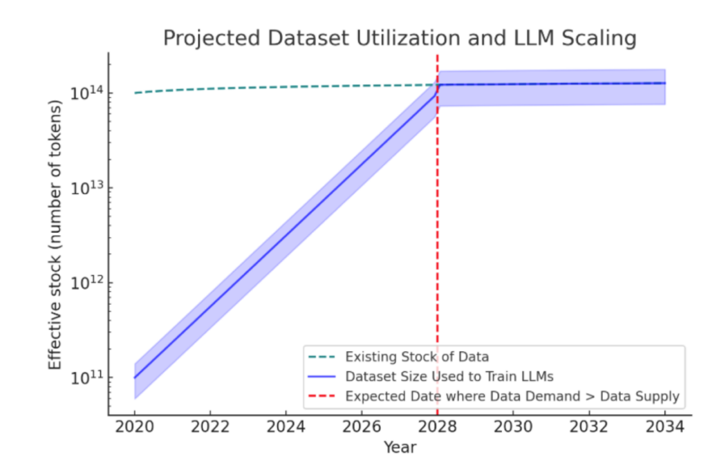
What happens if we run out of data?

Well, if we run out of data then we aren’t going to have anything new with which to train our language models. These models will then stop improving. If we want to pursue Artificial General Intelligence then we are going to have to come up with new ways of improving AI without just increasing the volume of real-world training data. 

One potential saviour is synthetic data which can be generated to mimic existing data and has already been used to improve the performance of models like Gemini and DBRX. 

Synthetic data beyond LLMs

Beyond overcoming data scarcity for large language models, synthetic data can be used in the following situations: 

• Sensitive Data — if we don’t want to share or use sensitive attributes, synthetic data can be generated which mimics the properties of these features while maintaining anonymity.
• Expensive data — if collecting data is expensive we can generate a large volume of synthetic data from a small amount of real-world data.
• Lack of data — datasets are biased when there is a disproportionately low number of individual data points from a particular group. Synthetic data can be used to balance a dataset. 

Imbalanced datasets

Imbalanced datasets can (*but not always*) be problematic as they may not contain enough information to effectively train a predictive model. For example, if a dataset contains many more men than women, our model may be biased towards recognising men and misclassify future female samples as men. 

In this article we show the imbalance in the popular UCI Adult dataset [2], and how we can use a variational auto-encoder to generate Synthetic Data to improve classification on this example. 

We first download the Adult dataset. This dataset contains features such as age, education and occupation which can be used to predict the target outcome ‘income’. 

# Download dataset into a dataframe
url = "https://archive.ics.uci.edu/ml/machine-learning-databases/adult/adult.data"
columns = [
   "age", "workclass", "fnlwgt", "education", "education-num", "marital-status",
   "occupation", "relationship", "race", "sex", "capital-gain",
   "capital-loss", "hours-per-week", "native-country", "income"
]
data = pd.read_csv(url, header=None, names=columns, na_values=" ?", skipinitialspace=True)

# Drop rows with missing values
data = data.dropna()

# Split into features and target
X = data.drop(columns=["income"])
y = data['income'].map({'>50K': 1, '<=50K': 0}).values

# Plot distribution of income
plt.figure(figsize=(8, 6))
plt.hist(data['income'], bins=2, edgecolor='black')
plt.title('Distribution of Income')
plt.xlabel('Income')
plt.ylabel('Frequency')
plt.show()

In the Adult dataset, income is a binary variable, representing individuals who earn above, and below, $50,000. We plot the distribution of income over the entire dataset below. We can see that the dataset is heavily imbalanced with a far larger number of individuals who earn less than $50,000. 

Despite this imbalance we can still train a machine learning classifier on the Adult dataset which we can use to determine whether unseen, or test, individuals should be classified as earning above, or below, 50k. 

# Preprocessing: One-hot encode categorical features, scale numerical features
numerical_features = ["age", "fnlwgt", "education-num", "capital-gain", "capital-loss", "hours-per-week"]
categorical_features = [
   "workclass", "education", "marital-status", "occupation", "relationship",
   "race", "sex", "native-country"
]

preprocessor = ColumnTransformer(
   transformers=[
       ("num", StandardScaler(), numerical_features),
       ("cat", OneHotEncoder(), categorical_features)
   ]
)

X_processed = preprocessor.fit_transform(X)

# Convert to numpy array for PyTorch compatibility
X_processed = X_processed.toarray().astype(np.float32)
y_processed = y.astype(np.float32)
# Split dataset in train and test sets
X_model_train, X_model_test, y_model_train, y_model_test = train_test_split(X_processed, y_processed, test_size=0.2, random_state=42)


rf_classifier = RandomForestClassifier(n_estimators=100, random_state=42)
rf_classifier.fit(X_model_train, y_model_train)

# Make predictions
y_pred = rf_classifier.predict(X_model_test)

# Display confusion matrix
plt.figure(figsize=(6, 4))
sns.heatmap(cm, annot=True, fmt="d", cmap="YlGnBu", xticklabels=["Negative", "Positive"], yticklabels=["Negative", "Positive"])
plt.xlabel("Predicted")
plt.ylabel("Actual")
plt.title("Confusion Matrix")
plt.show()

Printing out the confusion matrix of our classifier shows that our model performs fairly well despite the imbalance. Our model has an overall error rate of 16% but the error rate for the positive class (income > 50k) is 36% where the error rate for the negative class (income < 50k) is 8%. 

This discrepancy shows that the model is indeed biased towards the negative class. The model is frequently incorrectly classifying individuals who earn more than 50k as earning less than 50k. 

Below we show how we can use a Variational Autoencoder to generate synthetic data of the positive class to balance this dataset. We then train the same model using the synthetically balanced dataset and reduce model errors on the test set. 

How can we generate synthetic data?

There are lots of different methods for generating synthetic data. These can include more traditional methods such as SMOTE and Gaussian Noise which generate new data by modifying existing data. Alternatively Generative models such as Variational Autoencoders or General Adversarial networks are predisposed to generate new data as their architectures learn the distribution of real data and use these to generate synthetic samples.

In this tutorial we use a variational autoencoder to generate synthetic data.

Variational Autoencoders

Variational Autoencoders (VAEs) are great for synthetic data generation because they use real data to learn a continuous latent space. We can view this latent space as a magic bucket from which we can sample synthetic data which closely resembles existing data. The continuity of this space is one of their big selling points as it means the model generalises well and doesn’t just memorise the latent space of specific inputs.

A VAE consists of an encoder, which maps input data into a probability distribution (mean and variance) and a decoder, which reconstructs the data from the latent space. 

For that continuous latent space, VAEs use a reparameterization trick, where a random noise vector is scaled and shifted using the learned mean and variance, ensuring smooth and continuous representations in the latent space.

Below we construct a BasicVAE class which implements this process with a simple architecture.

•  The encoder compresses the input into a smaller, hidden representation, producing both a mean and log variance that define a Gaussian distribution aka creating our magic sampling bucket. Instead of directly sampling, the model applies the reparameterization trick to generate latent variables, which are then passed to the decoder. 
• The decoder reconstructs the original data from these latent variables, ensuring the generated data maintains characteristics of the original dataset. 

class BasicVAE(nn.Module):
   def __init__(self, input_dim, latent_dim):
       super(BasicVAE, self).__init__()
       # Encoder: Single small layer
       self.encoder = nn.Sequential(
           nn.Linear(input_dim, 8),
           nn.ReLU()
       )
       self.fc_mu = nn.Linear(8, latent_dim)
       self.fc_logvar = nn.Linear(8, latent_dim)
      
       # Decoder: Single small layer
       self.decoder = nn.Sequential(
           nn.Linear(latent_dim, 8),
           nn.ReLU(),
           nn.Linear(8, input_dim),
           nn.Sigmoid()  # Outputs values in range [0, 1]
       )

   def encode(self, x):
       h = self.encoder(x)
       mu = self.fc_mu(h)
       logvar = self.fc_logvar(h)
       return mu, logvar

   def reparameterize(self, mu, logvar):
       std = torch.exp(0.5 * logvar)
       eps = torch.randn_like(std)
       return mu + eps * std

   def decode(self, z):
       return self.decoder(z)

   def forward(self, x):
       mu, logvar = self.encode(x)
       z = self.reparameterize(mu, logvar)
       return self.decode(z), mu, logvar

Given our BasicVAE architecture we construct our loss functions and model training below. 

def vae_loss(recon_x, x, mu, logvar, tau=0.5, c=1.0):
   recon_loss = nn.MSELoss()(recon_x, x)
 
   # KL Divergence Loss
   kld_loss = -0.5 * torch.sum(1 + logvar - mu.pow(2) - logvar.exp())
   return recon_loss + kld_loss / x.size(0)

def train_vae(model, data_loader, epochs, learning_rate):
   optimizer = optim.Adam(model.parameters(), lr=learning_rate)
   model.train()
   losses = []
   reconstruction_mse = []

   for epoch in range(epochs):
       total_loss = 0
       total_mse = 0
       for batch in data_loader:
           batch_data = batch[0]
           optimizer.zero_grad()
           reconstructed, mu, logvar = model(batch_data)
           loss = vae_loss(reconstructed, batch_data, mu, logvar)
           loss.backward()
           optimizer.step()
           total_loss += loss.item()

           # Compute batch-wise MSE for comparison
           mse = nn.MSELoss()(reconstructed, batch_data).item()
           total_mse += mse

       losses.append(total_loss / len(data_loader))
       reconstruction_mse.append(total_mse / len(data_loader))
       print(f"Epoch {epoch+1}/{epochs}, Loss: {total_loss:.4f}, MSE: {total_mse:.4f}")
   return losses, reconstruction_mse

combined_data = np.concatenate([X_model_train.copy(), y_model_train.cop
y().reshape(26048,1)], axis=1)

# Train-test split
X_train, X_test = train_test_split(combined_data, test_size=0.2, random_state=42)

batch_size = 128

# Create DataLoaders
train_loader = DataLoader(TensorDataset(torch.tensor(X_train)), batch_size=batch_size, shuffle=True)
test_loader = DataLoader(TensorDataset(torch.tensor(X_test)), batch_size=batch_size, shuffle=False)

basic_vae = BasicVAE(input_dim=X_train.shape[1], latent_dim=8)

basic_losses, basic_mse = train_vae(
   basic_vae, train_loader, epochs=50, learning_rate=0.001,
)

# Visualize results
plt.figure(figsize=(12, 6))
plt.plot(basic_mse, label="Basic VAE")
plt.ylabel("Reconstruction MSE")
plt.title("Training Reconstruction MSE")
plt.legend()
plt.show()

vae_loss consists of two components: reconstruction loss, which measures how well the generated data matches the original input using Mean Squared Error (MSE), and KL divergence loss, which ensures that the learned latent space follows a normal distribution.

train_vae optimises the VAE using the Adam optimizer over multiple epochs. During training, the model takes mini-batches of data, reconstructs them, and computes the loss using vae_loss. These errors are then corrected via backpropagation where the model weights are updated. We train the model for 50 epochs and plot how the reconstruction mean squared error decreases over training.

We can see that our model learns quickly how to reconstruct our data, evidencing efficient learning. 

Now we have trained our BasicVAE to accurately reconstruct the Adult dataset we can now use it to generate synthetic data. We want to generate more samples of the positive class (individuals who earn over 50k) in order to balance out the classes and remove the bias from our model.

To do this we select all the samples from our VAE dataset where income is the positive class (earn more than 50k). We then encode these samples into the latent space. As we have only selected samples of the positive class to encode, this latent space will reflect properties of the positive class which we can sample from to create synthetic data. 

We sample 15000 new samples from this latent space and decode these latent vectors back into the input data space as our synthetic data points. 

# Create column names
col_number = sample_df.shape[1]
col_names = [str(i) for i in range(col_number)]
sample_df.columns = col_names

# Define the feature value to filter
feature_value = 1.0  # Specify the feature value - here we set the income to 1

# Set all income values to 1 : Over 50k
selected_samples = sample_df[sample_df[col_names[-1]] == feature_value]
selected_samples = selected_samples.values
selected_samples_tensor = torch.tensor(selected_samples, dtype=torch.float32)

basic_vae.eval()  # Set model to evaluation mode
with torch.no_grad():
   mu, logvar = basic_vae.encode(selected_samples_tensor)
   latent_vectors = basic_vae.reparameterize(mu, logvar)

# Compute the mean latent vector for this feature
mean_latent_vector = latent_vectors.mean(dim=0)


num_samples = 15000  # Number of new samples
latent_dim = 8
latent_samples = mean_latent_vector + 0.1 * torch.randn(num_samples, latent_dim)

with torch.no_grad():
   generated_samples = basic_vae.decode(latent_samples)

Now we have generated synthetic data of the positive class, we can combine this with the original training data to generate a balanced synthetic dataset. 

new_data = pd.DataFrame(generated_samples)

# Create column names
col_number = new_data.shape[1]
col_names = [str(i) for i in range(col_number)]
new_data.columns = col_names

X_synthetic = new_data.drop(col_names[-1],axis=1)
y_synthetic = np.asarray([1 for _ in range(0,X_synthetic.shape[0])])

X_synthetic_train = np.concatenate([X_model_train, X_synthetic.values], axis=0)
y_synthetic_train = np.concatenate([y_model_train, y_synthetic], axis=0)

mapping = {1: '>50K', 0: '<=50K'}
map_function = np.vectorize(lambda x: mapping[x])
# Apply mapping
y_mapped = map_function(y_synthetic_train)

plt.figure(figsize=(8, 6))
plt.hist(y_mapped, bins=2, edgecolor='black')
plt.title('Distribution of Income')
plt.xlabel('Income')
plt.ylabel('Frequency')
plt.show()

We can now use our balanced training synthetic dataset to retrain our random forest classifier. We can then evaluate this new model on the original test data to see how effective our synthetic data is at reducing the model bias.

rf_classifier = RandomForestClassifier(n_estimators=100, random_state=42)
rf_classifier.fit(X_synthetic_train, y_synthetic_train)

# Step 5: Make predictions
y_pred = rf_classifier.predict(X_model_test)

cm = confusion_matrix(y_model_test, y_pred)

# Create heatmap
plt.figure(figsize=(6, 4))
sns.heatmap(cm, annot=True, fmt="d", cmap="YlGnBu", xticklabels=["Negative", "Positive"], yticklabels=["Negative", "Positive"])
plt.xlabel("Predicted")
plt.ylabel("Actual")
plt.title("Confusion Matrix")
plt.show()

Our new classifier, trained on the balanced synthetic dataset makes fewer errors on the original test set than our original classifier trained on the imbalanced dataset and our error rate is now reduced to 14%.

However, we have not been able to reduce the discrepancy in errors by a significant amount, our error rate for the positive class is still 36%. This could be due to to the following reasons: 

• We have discussed how one of the benefits of VAEs is the learning of a continuous latent space. However, if the majority class dominates, the latent space might skew towards the majority class.
• The model may not have properly learned a distinct representation for the minority class due to the lack of data, making it hard to sample from that region accurately.

In this tutorial we have introduced and built a BasicVAE architecture which can be used to generate synthetic data which improves the classification accuracy on an imbalanced dataset. 

Follow for future articles where I will show how we can build more sophisticated VAE architectures which address the above problems with imbalanced sampling and more.

[1] Villalobos, P., Ho, A., Sevilla, J., Besiroglu, T., Heim, L., & Hobbhahn, M. (2024). Will we run out of data? Limits of LLM scaling based on human-generated data. arXiv preprint arXiv:2211.04325, 3.

[2] Becker, B. & Kohavi, R. (1996). Adult [Dataset]. UCI Machine Learning Repository. https://doi.org/10.24432/C5XW20.

The post The Next AI Revolution: A Tutorial Using VAEs to Generate High-Quality Synthetic Data appeared first on Towards Data Science.

​Leverage the BasicVAE architecture to generate synthetic data and improves the classification accuracy on an imbalanced dataset
The post The Next AI Revolution: A Tutorial Using VAEs to Generate High-Quality Synthetic Data appeared first on Towards Data Science.  Artificial Intelligence, Data Science, Hands On Tutorials, Imbalanced Data, Synthetic Data, Variational Autoencoder Towards Data ScienceRead More

Add to favorites