Part 3 of a hands-on guide to help you master MMM in pymc

What is this series about?

Welcome to part 3 of my series on marketing mix modelling (MMM), a hands-on guide to help you master MMM. Throughout this series, we’ll cover key topics such as model training, validation, calibration and budget optimisation, all using the powerful pymc-marketing python package. Whether you’re new to MMM or looking to sharpen your skills, this series will equip you with practical tools and insights to improve your marketing strategies.

If you missed part 2 check it out here:

Calibrating Marketing Mix Models In Python

Introduction

In the third instalment of the series we are going to cover how we can start to get business value from our marketing mix models by covering the following areas:

• Why do organisations want to optimise their marketing budgets?
• How can we use the outputs of our marketing mix model to optimise budgets?
• A python walkthrough demonstrating how to optimise budgets using pymc-marketing.

The full notebook can be found here:

pymc_marketing/notebooks/3. optimising budgets with marketing mix models (MMM) in python.ipynb at main · raz1470/pymc_marketing

1.0 Why do organisations want to optimise their marketing budgets?

This famous quote (from John Wanamaker I think?!) illustrates both the challenge and opportunity in marketing. While modern analytics have come a long way, the challenge remains relevant: understanding which parts of your marketing budget deliver value.

Marketing channels can vary significantly in terms of their performance and ROI due to several factors:

• Audience Reach and Engagement — Some channels are more effective at reaching specific prospects aligned to your target audience.
• Cost of Acquisition — The cost of reaching prospects differs between channels.
• Channel Saturation — Overuse of a marketing channel can lead to diminishing returns.

This variability creates the opportunity to ask critical questions that can transform your marketing strategy:

Effective budget optimisation is a critical component of modern marketing strategies. By leveraging the outputs of MMM, businesses can make informed decisions about where to allocate their resources for maximum impact. MMM provides insights into how various channels contribute to overall sales, allowing us to identify opportunities for improvement and optimisation. In the following sections, we will explore how we can translate MMM outputs into actionable budget allocation strategies.

2.1 Response curves

A response curve can translate the outputs of MMM into a comprehensive form, showing how sales responds to spend for each marketing channel.

Response curves alone are very powerful, allowing us to run what-if scenarios. Using the response curve above as an example, we could estimate how the sales contribution from social changes as we spend more. We can also visually see where diminishing returns starts to take effect. But what if we want to try and answer more complex what-if scenarios like optimising channel level budgets given a fixed overall budget? This is where linear programming comes in — Let’s explore this in the next section!

2.2 Linear programming

Linear programming is an optimisation method which can be used to find the optimal solution of a linear function given some constraints. It’s a very versatile tool from the operations research area but doesn’t often get the recognition it deserves. It is used to solve scheduling, transportation and resource allocation problems. We are going to explore how we can use it to optimise marketing budgets.

Let’s try and understand linear programming with a simple budget optimisation problem:

• Decision variables (x): These are the unknown quantities which we want to estimate optimal values for e.g. The marketing spend on each channel.
• Objective function (Z): The linear equation we are trying to minimise or maximise e.g. Maximising the sum of the sales contribution from each channel.
• Constraints: Some restrictions on the decision variables, usually represented by linear inequalities e.g. Total marketing budget is equal to £50m, Channel level budgets between £5m and £15m.

The intersection of all constraints forms a feasible region, which is the set of all possible solutions that satisfy the given constraints. The goal of linear programming is to find the point within the feasible region that optimises the objective function.

Given the saturation transformation we apply to each marketing channel, optimising channel level budgets is actually a non-linear programming problem. Sequential Least Squares Programming (SLSQP) is an algorithm used for solving non-linear programming problems. It allows for both equality and inequality constraints making it a sensible choice for our use case.

• Equality constraints e.g. Total marketing budget is equal to £50m
• Inequality constraints e.g. Channel level budgets between £5m and £15m

SciPy have a great implementation of SLSQP:

Optimization (scipy.optimize) – SciPy v1.14.1 Manual

The example below illustrates how we could use it:

from scipy.optimize import minimize

result = minimize(
    fun=objective_function,  # Define your ROI function here
    x0=initial_guess,        # Initial guesses for spends
    bounds=bounds,           # Channel-level budget constraints
    constraints=constraints, # Equality and inequality constraints
    method='SLSQP'
)
print(result)

Writing budget optimisation code from scratch is a complex but very rewarding exercise. Fortunately, the pymc-marketing team has done the heavy lifting, providing a robust framework for running budget optimisation scenarios. In the next section, we’ll explore how their package can streamline the budget allocation process and make it more accessible to analysts.

3.0 Python walkthrough

Now we understand how we can use the output of MMM to optimise budgets, let’s see how much value we can drive using our model from the last article! In this walkthrough we will cover:

• Simulating data
• Training the model
• Validating the model
• Response curves
• Budget optimisation

3.1 Simulating data

We are going to re-use the data-generating process from the first article. If you want a reminder on the data-generating process, take a look at the first article where we did a detailed walkthrough:

Mastering Marketing Mix Modelling In Python

np.random.seed(10)

# Set parameters for data generator
start_date = "2021-01-01"
periods = 52 * 3
channels = ["tv", "social", "search"]
adstock_alphas = [0.50, 0.25, 0.05]
saturation_lamdas = [1.5, 2.5, 3.5]
betas = [350, 150, 50]
spend_scalars = [10, 15, 20]

df = dg.data_generator(start_date, periods, channels, spend_scalars, adstock_alphas, saturation_lamdas, betas)

# Scale betas using maximum sales value - this is so it is comparable to the fitted beta from pymc (pymc does feature and target scaling using MaxAbsScaler from sklearn)
betas_scaled = [
    ((df["tv_sales"] / df["sales"].max()) / df["tv_saturated"]).mean(),
    ((df["social_sales"] / df["sales"].max()) / df["social_saturated"]).mean(),
    ((df["search_sales"] / df["sales"].max()) / df["search_saturated"]).mean()
]

# Calculate contributions
contributions = np.asarray([
    round((df["tv_sales"].sum() / df["sales"].sum()), 2),
    round((df["social_sales"].sum() / df["sales"].sum()), 2),
    round((df["search_sales"].sum() / df["sales"].sum()), 2),
    round((df["demand"].sum() / df["sales"].sum()), 2)
])

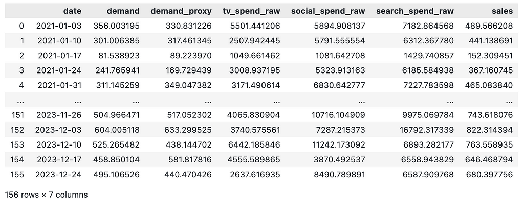
df[["date", "demand", "demand_proxy", "tv_spend_raw", "social_spend_raw", "search_spend_raw", "sales"]]

3.2 Training the model

We are now going to re-train the model from the first article. We will prepare the training data in the same way as last time by:

• Splitting data into features and target.
• Creating indices for train and out-of-time slices.

However, as the focus of this article is not on model calibration, we are going to include demand as a control variable rather than demand_proxy. This means the model will be very well calibrated — Although this isn’t very realistic, it will give us some good results to illustrate how we can optimise budgets.

# set date column
date_col = "date"

# set outcome column
y_col = "sales"

# set marketing variables
channel_cols = ["tv_spend_raw",
                "social_spend_raw",
                "search_spend_raw"]

# set control variables
control_cols = ["demand"]

# create arrays
X = df[[date_col] + channel_cols + control_cols]
y = df[y_col]

# set test (out-of-sample) length
test_len = 8

# create train and test indexs
train_idx = slice(0, len(df) - test_len)
out_of_time_idx = slice(len(df) - test_len, len(df))

mmm_default = MMM(
    adstock=GeometricAdstock(l_max=8),
    saturation=LogisticSaturation(),
    date_column=date_col,
    channel_columns=channel_cols,
    control_columns=control_cols,
)

fit_kwargs = {
    "tune": 1_000,
    "chains": 4,
    "draws": 1_000,
    "target_accept": 0.9,
}

mmm_default.fit(X[train_idx], y[train_idx], **fit_kwargs)

3.3 Validating the model

Before we get into the optimisation, lets check our model fits well. First we check the true contributions:

channels = np.array(["tv", "social", "search", "demand"])

true_contributions = pd.DataFrame({'Channels': channels, 'Contributions': contributions})
true_contributions= true_contributions.sort_values(by='Contributions', ascending=False).reset_index(drop=True)
true_contributions = true_contributions.style.bar(subset=['Contributions'], color='lightblue')

true_contributions

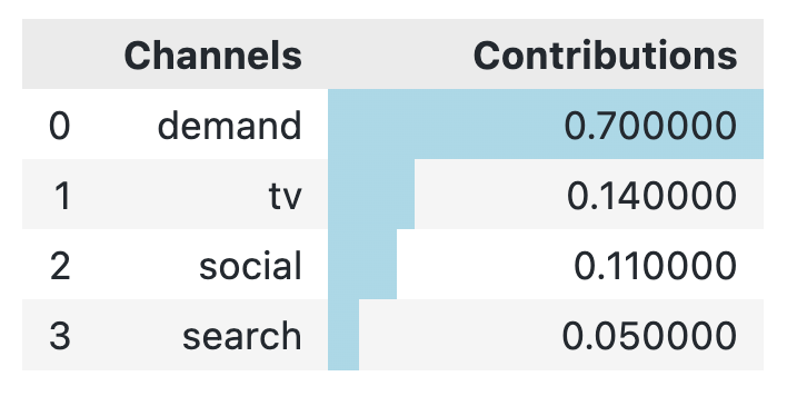
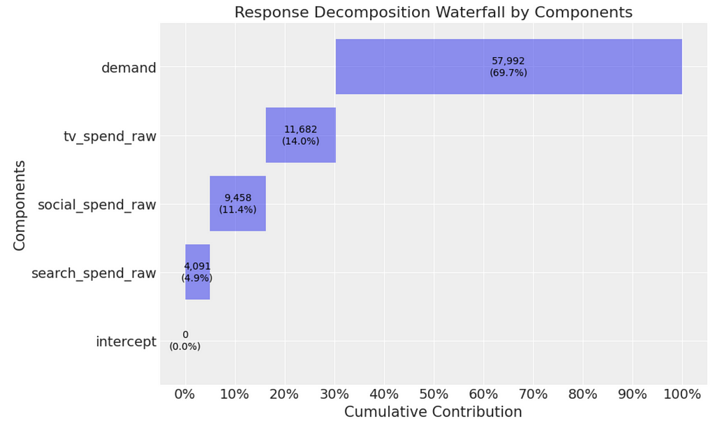
As expected, our model aligns very closely to the true contributions:

mmm_default.plot_waterfall_components_decomposition(figsize=(10,6));

3.4 Response curves

Before we get into the budget optimisation, let’s take a look at the response curves. There are two ways to look at response curves in the pymc-marketing package:

1. Direct response curves
2. Cost share response curves

Let’s start with the direct response curves. In the direct response curves we simply create a scatter plot of weekly spend against weekly contribution for each channel.

Below we plot the direct response curves:

fig = mmm_default.plot_direct_contribution_curves(show_fit=True, xlim_max=1.2)
[ax.set(xlabel="spend") for ax in fig.axes];

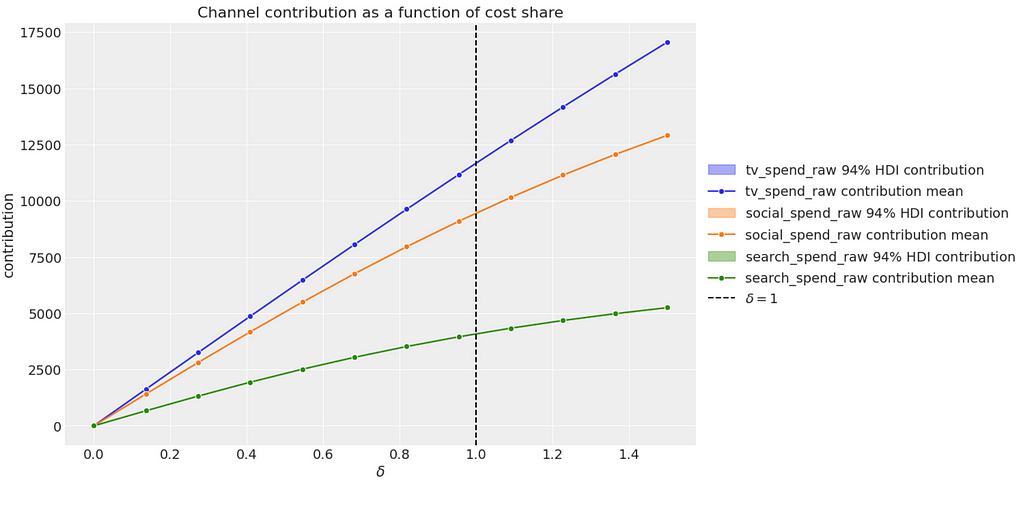
The cost share response curves are an alternative way of comparing the effectiveness of channels. When δ = 1.0, the channel spend remains at the same level as the training data. When δ = 1.2, the channel spend is increased by 20%.

Below we plot the cost share response curves:

mmm_default.plot_channel_contributions_grid(start=0, stop=1.5, num=12, figsize=(15, 7));

We can also change the x-axis to show absolute spend values:

mmm_default.plot_channel_contributions_grid(start=0, stop=1.5, num=12, absolute_xrange=True, figsize=(15, 7));

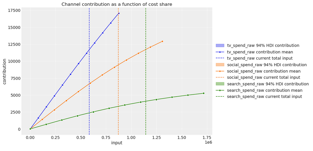
The response curves are great tools to help think about planning future marketing budgets at a channel level. Next lets put them to action and run some budget optimisation scenarios!

3.5 Budget optimisation

To begin with let’s set a couple of parameters:

• perc_change: This is used to set the constraint around min and max spend on each channel. This constraint helps us keep the scenario realistic and means we don’t extrapolate response curves too far outside of what the model has seen in training.
• budget_len: This is the length of the budget scenario in weeks.

We will start by using the desired length of the budget scenario to select the most recent period of data.

perc_change = 0.20
budget_len = 12
budget_idx = slice(len(df) - test_len, len(df))
recent_period = X[budget_idx][channel_cols]

recent_period

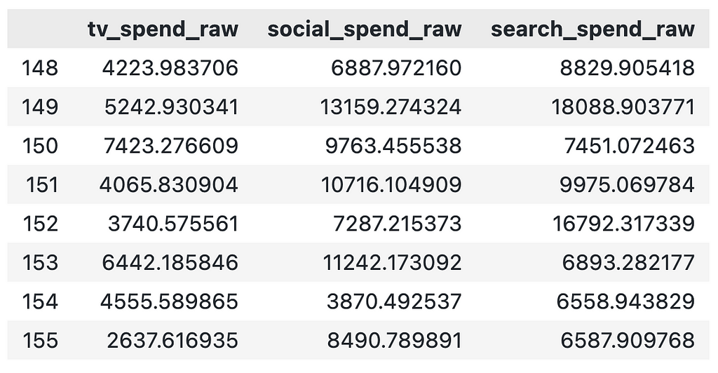
We then use this recent period to set overall budget constraints and channel constraints at a weekly level:

# set overall budget constraint (to the nearest £1k)
budget = round(recent_period.sum(axis=0).sum() / budget_len, -3)

# record the current budget split by channel
current_budget_split = round(recent_period.mean() / recent_period.mean().sum(), 2)

# set channel level constraints
lower_bounds = round(recent_period.min(axis=0) * (1 - perc_change))
upper_bounds = round(recent_period.max(axis=0) * (1 + perc_change))

budget_bounds = {
    channel: [lower_bounds[channel], upper_bounds[channel]]
    for channel in channel_cols
}

print(f'Overall budget constraint: {budget}')
print('Channel constraints:')
for channel, bounds in budget_bounds.items():
    print(f'  {channel}: Lower Bound = {bounds[0]}, Upper Bound = {bounds[1]}')

Now it’s time to run our scenario! We feed in the relevant data and parameters and get back the optimal spend. We compare it to taking the total budget and splitting it by the current budget split proportions (which we have called actual spend).

model_granularity = "weekly"

# run scenario
allocation_strategy, optimization_result = mmm_default.optimize_budget(
    budget=budget,
    num_periods=budget_len,
    budget_bounds=budget_bounds,
    minimize_kwargs={
        "method": "SLSQP",
        "options": {"ftol": 1e-9, "maxiter": 5_000},
    },
)

response = mmm_default.sample_response_distribution(
    allocation_strategy=allocation_strategy,
    time_granularity=model_granularity,
    num_periods=budget_len,
    noise_level=0.05,
)

# extract optimal spend
opt_spend = pd.Series(allocation_strategy, index=recent_period.mean().index).to_frame(name="opt_spend")
opt_spend["avg_spend"] = budget * current_budget_split

# plot actual vs optimal spend
fig, ax = plt.subplots(figsize=(9, 4))
opt_spend.plot(kind='barh', ax=ax, color=['blue', 'orange'])

plt.xlabel("Spend")
plt.ylabel("Channel")
plt.title("Actual vs Optimal Spend by Channel")
plt.legend(["Optimal Spend", "Actual Spend"])
plt.legend(["Optimal Spend", "Actual Spend"], loc='lower right', bbox_to_anchor=(1.5, 0.0))

plt.show()

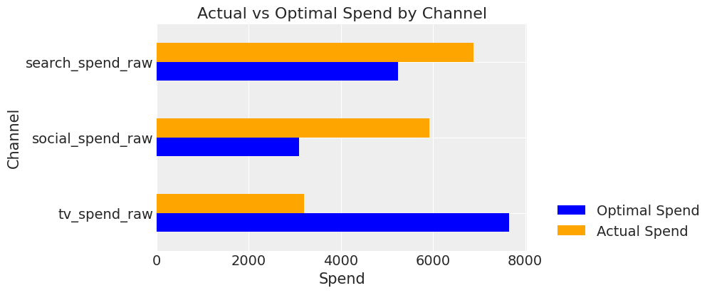
We can see the suggestion is to move budget from digital channels to TV. But what is the impact on sales?

To calculate the contribution of the optimal spend we need to feed in the new spend value per channel plus any other variables in the model. We only have demand, so we feed in the mean value from the recent period for this. We will also calculate the contribution of the average spend in the same way.

# create dataframe with optimal spend
last_date = mmm_default.X["date"].max()
new_dates = pd.date_range(start=last_date, periods=1 + budget_len, freq="W-MON")[1:]
budget_scenario_opt = pd.DataFrame({"date": new_dates,})
budget_scenario_opt["tv_spend_raw"] = opt_spend["opt_spend"]["tv_spend_raw"]
budget_scenario_opt["social_spend_raw"] = opt_spend["opt_spend"]["social_spend_raw"]
budget_scenario_opt["search_spend_raw"] = opt_spend["opt_spend"]["search_spend_raw"]
budget_scenario_opt["demand"] = X[budget_idx][control_cols].mean()[0]

# calculate overall contribution
scenario_contrib_opt = mmm_default.sample_posterior_predictive(
    X_pred=budget_scenario_opt, extend_idata=False
)

opt_contrib = scenario_contrib_opt.mean(dim="sample").sum()["y"].values

# create dataframe with avg spend
last_date = mmm_default.X["date"].max()
new_dates = pd.date_range(start=last_date, periods=1 + budget_len, freq="W-MON")[1:]
budget_scenario_avg = pd.DataFrame({"date": new_dates,})
budget_scenario_avg["tv_spend_raw"] = opt_spend["avg_spend"]["tv_spend_raw"]
budget_scenario_avg["social_spend_raw"] = opt_spend["avg_spend"]["social_spend_raw"]
budget_scenario_avg["search_spend_raw"] = opt_spend["avg_spend"]["search_spend_raw"]
budget_scenario_avg["demand"] = X[budget_idx][control_cols].mean()[0]

# calculate overall contribution
scenario_contrib_avg  = mmm_default.sample_posterior_predictive(
    X_pred=budget_scenario_avg , extend_idata=False
)

avg_contrib = scenario_contrib_avg.mean(dim="sample").sum()["y"].values

# calculate % increase in sales
print(f'% increase in sales: {round((opt_contrib / avg_contrib) - 1, 2)}')

The optimal spend gives us a 6% increase in sales! That’s impressive especially given we have fixed the overall budget!

Closing thoughts

Today we have seen how powerful budget optimisation can be. It can help organisations with monthly/quarterly/yearly budget planning and forecasting. As always the key to making good recommendations comes back to having a robust, well calibrated model.

I hope you enjoyed the third instalment! That’s it for this series on mastering MMM. However, stay tuned if you want to learn about the complex topic of measuring long-term brand building effects!

---

Optimising Budgets With Marketing Mix Models In Python was originally published in Towards Data Science on Medium, where people are continuing the conversation by highlighting and responding to this story.

​Part 3 of a hands-on guide to help you master MMM in pymcPhoto by Towfiqu barbhuiya on UnsplashWhat is this series about?Welcome to part 3 of my series on marketing mix modelling (MMM), a hands-on guide to help you master MMM. Throughout this series, we’ll cover key topics such as model training, validation, calibration and budget optimisation, all using the powerful pymc-marketing python package. Whether you’re new to MMM or looking to sharpen your skills, this series will equip you with practical tools and insights to improve your marketing strategies.If you missed part 2 check it out here:Calibrating Marketing Mix Models In PythonIntroductionIn the third instalment of the series we are going to cover how we can start to get business value from our marketing mix models by covering the following areas:Why do organisations want to optimise their marketing budgets?How can we use the outputs of our marketing mix model to optimise budgets?A python walkthrough demonstrating how to optimise budgets using pymc-marketing.The full notebook can be found here:pymc_marketing/notebooks/3. optimising budgets with marketing mix models (MMM) in python.ipynb at main · raz1470/pymc_marketing1.0 Why do organisations want to optimise their marketing budgets?User generated imageThis famous quote (from John Wanamaker I think?!) illustrates both the challenge and opportunity in marketing. While modern analytics have come a long way, the challenge remains relevant: understanding which parts of your marketing budget deliver value.Marketing channels can vary significantly in terms of their performance and ROI due to several factors:Audience Reach and Engagement — Some channels are more effective at reaching specific prospects aligned to your target audience.Cost of Acquisition — The cost of reaching prospects differs between channels.Channel Saturation — Overuse of a marketing channel can lead to diminishing returns.This variability creates the opportunity to ask critical questions that can transform your marketing strategy:User generated imageEffective budget optimisation is a critical component of modern marketing strategies. By leveraging the outputs of MMM, businesses can make informed decisions about where to allocate their resources for maximum impact. MMM provides insights into how various channels contribute to overall sales, allowing us to identify opportunities for improvement and optimisation. In the following sections, we will explore how we can translate MMM outputs into actionable budget allocation strategies.2.1 Response curvesA response curve can translate the outputs of MMM into a comprehensive form, showing how sales responds to spend for each marketing channel.User generated imageResponse curves alone are very powerful, allowing us to run what-if scenarios. Using the response curve above as an example, we could estimate how the sales contribution from social changes as we spend more. We can also visually see where diminishing returns starts to take effect. But what if we want to try and answer more complex what-if scenarios like optimising channel level budgets given a fixed overall budget? This is where linear programming comes in — Let’s explore this in the next section!2.2 Linear programmingLinear programming is an optimisation method which can be used to find the optimal solution of a linear function given some constraints. It’s a very versatile tool from the operations research area but doesn’t often get the recognition it deserves. It is used to solve scheduling, transportation and resource allocation problems. We are going to explore how we can use it to optimise marketing budgets.Let’s try and understand linear programming with a simple budget optimisation problem:Decision variables (x): These are the unknown quantities which we want to estimate optimal values for e.g. The marketing spend on each channel.Objective function (Z): The linear equation we are trying to minimise or maximise e.g. Maximising the sum of the sales contribution from each channel.Constraints: Some restrictions on the decision variables, usually represented by linear inequalities e.g. Total marketing budget is equal to £50m, Channel level budgets between £5m and £15m.User generated imageThe intersection of all constraints forms a feasible region, which is the set of all possible solutions that satisfy the given constraints. The goal of linear programming is to find the point within the feasible region that optimises the objective function.Given the saturation transformation we apply to each marketing channel, optimising channel level budgets is actually a non-linear programming problem. Sequential Least Squares Programming (SLSQP) is an algorithm used for solving non-linear programming problems. It allows for both equality and inequality constraints making it a sensible choice for our use case.Equality constraints e.g. Total marketing budget is equal to £50mInequality constraints e.g. Channel level budgets between £5m and £15mSciPy have a great implementation of SLSQP:Optimization (scipy.optimize) – SciPy v1.14.1 ManualThe example below illustrates how we could use it:from scipy.optimize import minimizeresult = minimize( fun=objective_function, # Define your ROI function here x0=initial_guess, # Initial guesses for spends bounds=bounds, # Channel-level budget constraints constraints=constraints, # Equality and inequality constraints method=’SLSQP’)print(result)Writing budget optimisation code from scratch is a complex but very rewarding exercise. Fortunately, the pymc-marketing team has done the heavy lifting, providing a robust framework for running budget optimisation scenarios. In the next section, we’ll explore how their package can streamline the budget allocation process and make it more accessible to analysts.3.0 Python walkthroughNow we understand how we can use the output of MMM to optimise budgets, let’s see how much value we can drive using our model from the last article! In this walkthrough we will cover:Simulating dataTraining the modelValidating the modelResponse curvesBudget optimisation3.1 Simulating dataWe are going to re-use the data-generating process from the first article. If you want a reminder on the data-generating process, take a look at the first article where we did a detailed walkthrough:Mastering Marketing Mix Modelling In Pythonnp.random.seed(10)# Set parameters for data generatorstart_date = “2021-01-01″periods = 52 * 3channels = [“tv”, “social”, “search”]adstock_alphas = [0.50, 0.25, 0.05]saturation_lamdas = [1.5, 2.5, 3.5]betas = [350, 150, 50]spend_scalars = [10, 15, 20]df = dg.data_generator(start_date, periods, channels, spend_scalars, adstock_alphas, saturation_lamdas, betas)# Scale betas using maximum sales value – this is so it is comparable to the fitted beta from pymc (pymc does feature and target scaling using MaxAbsScaler from sklearn)betas_scaled = [ ((df[“tv_sales”] / df[“sales”].max()) / df[“tv_saturated”]).mean(), ((df[“social_sales”] / df[“sales”].max()) / df[“social_saturated”]).mean(), ((df[“search_sales”] / df[“sales”].max()) / df[“search_saturated”]).mean()]# Calculate contributionscontributions = np.asarray([ round((df[“tv_sales”].sum() / df[“sales”].sum()), 2), round((df[“social_sales”].sum() / df[“sales”].sum()), 2), round((df[“search_sales”].sum() / df[“sales”].sum()), 2), round((df[“demand”].sum() / df[“sales”].sum()), 2)])df[[“date”, “demand”, “demand_proxy”, “tv_spend_raw”, “social_spend_raw”, “search_spend_raw”, “sales”]]User generated image3.2 Training the modelWe are now going to re-train the model from the first article. We will prepare the training data in the same way as last time by:Splitting data into features and target.Creating indices for train and out-of-time slices.However, as the focus of this article is not on model calibration, we are going to include demand as a control variable rather than demand_proxy. This means the model will be very well calibrated — Although this isn’t very realistic, it will give us some good results to illustrate how we can optimise budgets.# set date columndate_col = “date”# set outcome columny_col = “sales”# set marketing variableschannel_cols = [“tv_spend_raw”, “social_spend_raw”, “search_spend_raw”]# set control variablescontrol_cols = [“demand”]# create arraysX = df[[date_col] + channel_cols + control_cols]y = df[y_col]# set test (out-of-sample) lengthtest_len = 8# create train and test indexstrain_idx = slice(0, len(df) – test_len)out_of_time_idx = slice(len(df) – test_len, len(df))mmm_default = MMM( adstock=GeometricAdstock(l_max=8), saturation=LogisticSaturation(), date_column=date_col, channel_columns=channel_cols, control_columns=control_cols,)fit_kwargs = { “tune”: 1_000, “chains”: 4, “draws”: 1_000, “target_accept”: 0.9,}mmm_default.fit(X[train_idx], y[train_idx], **fit_kwargs)3.3 Validating the modelBefore we get into the optimisation, lets check our model fits well. First we check the true contributions:channels = np.array([“tv”, “social”, “search”, “demand”])true_contributions = pd.DataFrame({‘Channels’: channels, ‘Contributions’: contributions})true_contributions= true_contributions.sort_values(by=’Contributions’, ascending=False).reset_index(drop=True)true_contributions = true_contributions.style.bar(subset=[‘Contributions’], color=’lightblue’)true_contributionsUser generated imageAs expected, our model aligns very closely to the true contributions:mmm_default.plot_waterfall_components_decomposition(figsize=(10,6));User generated image3.4 Response curvesBefore we get into the budget optimisation, let’s take a look at the response curves. There are two ways to look at response curves in the pymc-marketing package:Direct response curvesCost share response curvesLet’s start with the direct response curves. In the direct response curves we simply create a scatter plot of weekly spend against weekly contribution for each channel.Below we plot the direct response curves:fig = mmm_default.plot_direct_contribution_curves(show_fit=True, xlim_max=1.2)[ax.set(xlabel=”spend”) for ax in fig.axes];User generated imageThe cost share response curves are an alternative way of comparing the effectiveness of channels. When δ = 1.0, the channel spend remains at the same level as the training data. When δ = 1.2, the channel spend is increased by 20%.Below we plot the cost share response curves:mmm_default.plot_channel_contributions_grid(start=0, stop=1.5, num=12, figsize=(15, 7));user generated imageWe can also change the x-axis to show absolute spend values:mmm_default.plot_channel_contributions_grid(start=0, stop=1.5, num=12, absolute_xrange=True, figsize=(15, 7));user generated imageThe response curves are great tools to help think about planning future marketing budgets at a channel level. Next lets put them to action and run some budget optimisation scenarios!3.5 Budget optimisationTo begin with let’s set a couple of parameters:perc_change: This is used to set the constraint around min and max spend on each channel. This constraint helps us keep the scenario realistic and means we don’t extrapolate response curves too far outside of what the model has seen in training.budget_len: This is the length of the budget scenario in weeks.We will start by using the desired length of the budget scenario to select the most recent period of data.perc_change = 0.20budget_len = 12budget_idx = slice(len(df) – test_len, len(df))recent_period = X[budget_idx][channel_cols]recent_periodUser generated imageWe then use this recent period to set overall budget constraints and channel constraints at a weekly level:# set overall budget constraint (to the nearest £1k)budget = round(recent_period.sum(axis=0).sum() / budget_len, -3)# record the current budget split by channelcurrent_budget_split = round(recent_period.mean() / recent_period.mean().sum(), 2)# set channel level constraintslower_bounds = round(recent_period.min(axis=0) * (1 – perc_change))upper_bounds = round(recent_period.max(axis=0) * (1 + perc_change))budget_bounds = { channel: [lower_bounds[channel], upper_bounds[channel]] for channel in channel_cols}print(f’Overall budget constraint: {budget}’)print(‘Channel constraints:’)for channel, bounds in budget_bounds.items(): print(f’ {channel}: Lower Bound = {bounds[0]}, Upper Bound = {bounds[1]}’)User generated imageNow it’s time to run our scenario! We feed in the relevant data and parameters and get back the optimal spend. We compare it to taking the total budget and splitting it by the current budget split proportions (which we have called actual spend).model_granularity = “weekly”# run scenarioallocation_strategy, optimization_result = mmm_default.optimize_budget( budget=budget, num_periods=budget_len, budget_bounds=budget_bounds, minimize_kwargs={ “method”: “SLSQP”, “options”: {“ftol”: 1e-9, “maxiter”: 5_000}, },)response = mmm_default.sample_response_distribution( allocation_strategy=allocation_strategy, time_granularity=model_granularity, num_periods=budget_len, noise_level=0.05,)# extract optimal spendopt_spend = pd.Series(allocation_strategy, index=recent_period.mean().index).to_frame(name=”opt_spend”)opt_spend[“avg_spend”] = budget * current_budget_split# plot actual vs optimal spendfig, ax = plt.subplots(figsize=(9, 4))opt_spend.plot(kind=’barh’, ax=ax, color=[‘blue’, ‘orange’])plt.xlabel(“Spend”)plt.ylabel(“Channel”)plt.title(“Actual vs Optimal Spend by Channel”)plt.legend([“Optimal Spend”, “Actual Spend”])plt.legend([“Optimal Spend”, “Actual Spend”], loc=’lower right’, bbox_to_anchor=(1.5, 0.0))plt.show()User generated imageWe can see the suggestion is to move budget from digital channels to TV. But what is the impact on sales?To calculate the contribution of the optimal spend we need to feed in the new spend value per channel plus any other variables in the model. We only have demand, so we feed in the mean value from the recent period for this. We will also calculate the contribution of the average spend in the same way.# create dataframe with optimal spendlast_date = mmm_default.X[“date”].max()new_dates = pd.date_range(start=last_date, periods=1 + budget_len, freq=”W-MON”)[1:]budget_scenario_opt = pd.DataFrame({“date”: new_dates,})budget_scenario_opt[“tv_spend_raw”] = opt_spend[“opt_spend”][“tv_spend_raw”]budget_scenario_opt[“social_spend_raw”] = opt_spend[“opt_spend”][“social_spend_raw”]budget_scenario_opt[“search_spend_raw”] = opt_spend[“opt_spend”][“search_spend_raw”]budget_scenario_opt[“demand”] = X[budget_idx][control_cols].mean()[0]# calculate overall contributionscenario_contrib_opt = mmm_default.sample_posterior_predictive( X_pred=budget_scenario_opt, extend_idata=False)opt_contrib = scenario_contrib_opt.mean(dim=”sample”).sum()[“y”].values# create dataframe with avg spendlast_date = mmm_default.X[“date”].max()new_dates = pd.date_range(start=last_date, periods=1 + budget_len, freq=”W-MON”)[1:]budget_scenario_avg = pd.DataFrame({“date”: new_dates,})budget_scenario_avg[“tv_spend_raw”] = opt_spend[“avg_spend”][“tv_spend_raw”]budget_scenario_avg[“social_spend_raw”] = opt_spend[“avg_spend”][“social_spend_raw”]budget_scenario_avg[“search_spend_raw”] = opt_spend[“avg_spend”][“search_spend_raw”]budget_scenario_avg[“demand”] = X[budget_idx][control_cols].mean()[0]# calculate overall contributionscenario_contrib_avg = mmm_default.sample_posterior_predictive( X_pred=budget_scenario_avg , extend_idata=False)avg_contrib = scenario_contrib_avg.mean(dim=”sample”).sum()[“y”].values# calculate % increase in salesprint(f’% increase in sales: {round((opt_contrib / avg_contrib) – 1, 2)}’)User generated imageThe optimal spend gives us a 6% increase in sales! That’s impressive especially given we have fixed the overall budget!Closing thoughtsToday we have seen how powerful budget optimisation can be. It can help organisations with monthly/quarterly/yearly budget planning and forecasting. As always the key to making good recommendations comes back to having a robust, well calibrated model.I hope you enjoyed the third instalment! That’s it for this series on mastering MMM. However, stay tuned if you want to learn about the complex topic of measuring long-term brand building effects!Optimising Budgets With Marketing Mix Models In Python was originally published in Towards Data Science on Medium, where people are continuing the conversation by highlighting and responding to this story.  programming, marketing, data-science, causal-inference, marketing-mix-modeling Towards Data Science – MediumRead More

Add to favorites