LossVal Explained: Efficient Data Valuation for Neural Networks
How to exploit the loss function to efficiently estimate the importance of your training data

This blog post summarizes and explains our paper “LossVal: Efficient Data Valuation for Neural Networks”.
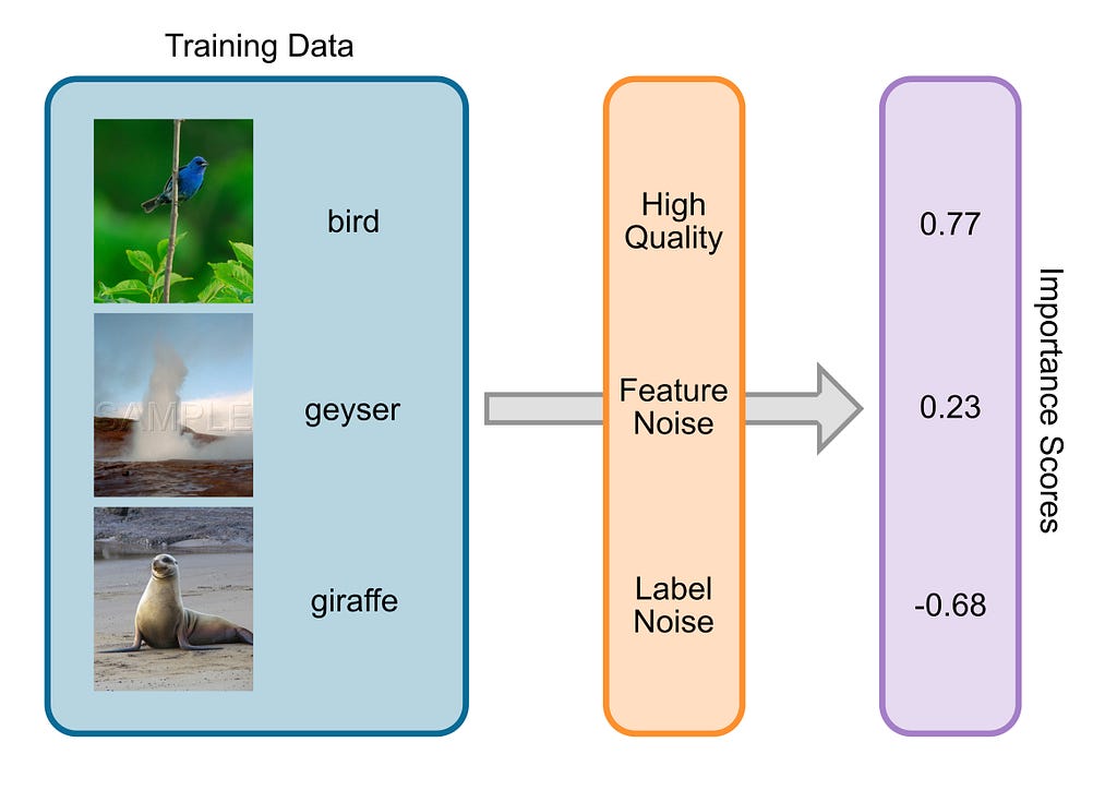
Not all data is created equal: Some training data points influence the training of a machine learning model much more than others. Understanding the influence of each data point is often highly inefficient and often relies on repeated retraining of the model. LossVal presents a new approach to this, that efficiently integrates the Data Valuation process into the loss function of an artificial neural network.
What is Data Valuation?
Machine Learning models are often trained with large datasets. In most cases, not all training samples in such a dataset are equally helpful or informative for the model. For example, if a data point is noisy or has a wrong label, it is less informative for your machine learning model. For one of the tasks in our paper, we trained a machine-learning model on a vehicle crash test dataset to predict how harmful a crash would be for an occupant, based on some vehicle parameters. Some of the data points are from cars of the 80s and 90s! You can imagine, that very old cars may be less important for the model’s predictions on modern cars.
The process of understanding the effect of each training sample on the machine-learning model is called Data Valuation, where an importance score is assigned to each training sample. Data Valuation is a growing field connected to data markets, explainable AI, active learning, and many more. Many approaches have been proposed, like Data Shapley, Influence Functions, or LAVA. To learn more about this, you can check out my recent blog post that presents different Data Valuation methods and applications.
LossVal
The basic idea behind LossVal is to “learn” the importance score of each sample while training the model, similar to how the model weights are learned. This saves us from rerunning the training of the model multiple times and from having to track all model weight updates during the training.
To achieve this, we can modify standard loss functions like means squared error (MSE) and cross-entropy loss. We incorporate instance-based weights into the loss and multiply it by a weighted distance function. In general, the LossVal loss functions have the following form:
https://medium.com/media/b2524fa59ac79e1633ebd65045e6bca4/href
where ℒ indicates the weighted target loss (weighted MSE or cross-entropy) and OT indicates a weighted distribution distance (OT stands for optimal transport). This results in new loss functions that can be used like any other loss function for training a neural network. However, during each training step, the weights w in the loss are updated using the gradient descent.
We demonstrate this for regression tasks using the MSE and for classification using the cross-entropy loss. Afterward, we take a closer look at the distribution distance OT.
LossVal for Regression
Let’s start with the MSE. The standard MSE is the squared difference between the model prediction ŷ and the correct prediction y (with n being the index of the training sample):
https://medium.com/media/a5ae23d613cad57cebf9edf35066a2fd/href
For LossVal, we modify the MSE in two steps: First, a weight wₙ is included for each training instance n. Second, the whole MSE is multiplied with a weighted distribution distance function.
https://medium.com/media/f99d0bf5c6397a1413af6e7c0cd1bbc2/href
LossVal for Classification
The cross-entropy loss is typically expressed like this:
https://medium.com/media/afea75b0dea4cc524a32636c32013d1d/href
We can modify the cross-entropy loss in the same way as the MSE:
https://medium.com/media/6a02a1027b1f9d2dc2b2adb276534e71/href
The Optimal Transport Distance
The optimal transport distance is the minimum effort you need to transform one distribution into another. It is also known as the earth mover distance, coming from the analogy of the fastest way to fill a hole with a pile of dirt. OT can be defined as:
https://medium.com/media/db5f30eeb15fc7b2d6fbd4340909d5da/href
where c is the cost of moving point xₙ to xⱼ. Each γ is a possible transport plan, defining how the points are moved. The optimal transport plan is the γ* with the least effort involved (the smallest distribution distance). Note that we include the weights w in the cost function via joint distribution Π(w, 1). In other words, OTᵥᵥ is the weighted distance between the training and the validation set. You can find an in-depth explanation for optimal transport here.
In a more practical sense, minimizing OTᵥᵥ by changing the weights will assign higher weights to the training data points similar to the validation data. Effectively, noisy samples get a smaller weight.
Implementation
Our implementation and all data are available on GitHub. The code below shows the implementation of LossVal for the mean squared error.
def LossVal_mse(train_X: torch.Tensor,
                train_y_true: torch.Tensor, train_y_pred: torch.Tensor,
                val_X: torch.Tensor, sample_ids: torch.Tensor
                weights: torch.Tensor, device: torch.device) -> torch.Tensor:
    weights = weights.index_select(0, sample_ids)  # Select the weights corresponding to the sample_ids

    # Step 1: Compute the weighted mse loss
    loss = torch.sum((train_y_true - train_y_pred) ** 2, dim=1)
    weighted_loss = torch.sum(weights @ loss)  # Loss is a vector, weights is a matrix

    # Step 2: Compute the Sinkhorn distance between the training and validation distributions
    sinkhorn_distance = SamplesLoss(loss="sinkhorn")
    dist_loss = sinkhorn_distance(weights, train_X, torch.ones(val_X.shape[0], requires_grad=True).to(device), val_X)

    # Step 3: Combine mse and Sinkhorn distance
    return weighted_loss * dist_loss**2
This loss function works like any other loss function in pytorch, with some peculiarities: the parameters include the validation set, sample weights, and the indices of the samples in the batch. This is necessary to select the correct weights for the batched samples for calculating the weighted loss. Keep in mind that this implementation relies on the automatic gradient calculation of pytorch. That means the sample weights vector needs to be part of the model parameters. This way, the optimization of the weights profits from the optimizer implementation, like Adam. Alternatively, one could also update the weights per hand, using the gradient of the loss with respect to each weight i. The implementation for cross-entropy works equivalently, but you need to replace line 8.
But does it work?

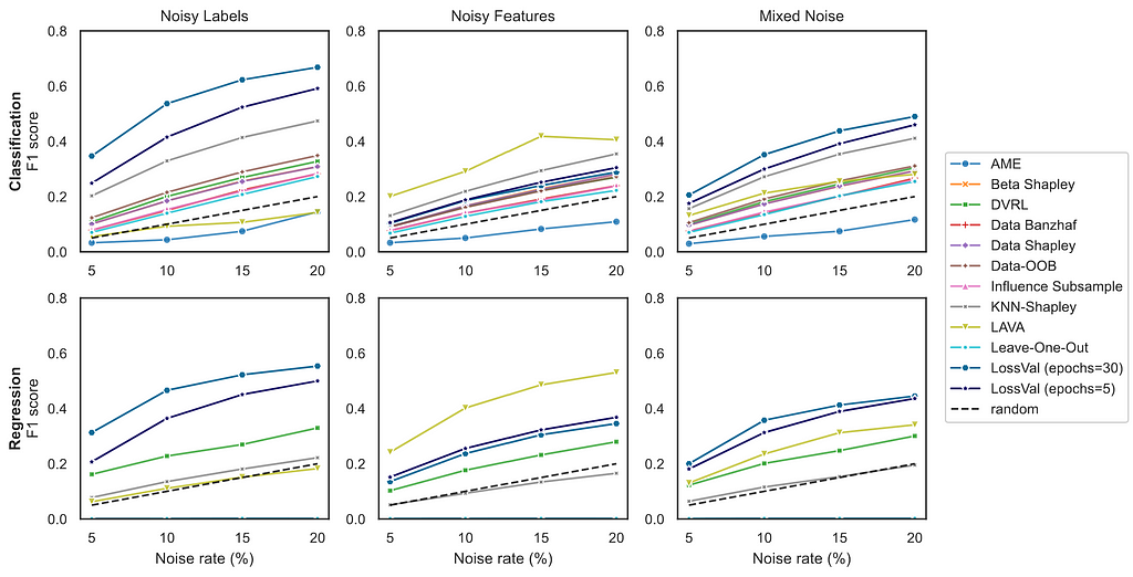
The graphic above shows the comparison between different Data Valuation approaches on the noisy sample detection task. This task is defined by the OpenDataVal benchmark. First, noise is added to p% of the training data, then the Data Valuation is used to find the noisy samples. Better methods will find more of the noisy samples, hence achieving a higher F1 score. The graph above shows the average over 6 datasets for classification and 6 datasets for regression. We tested 3 different noise types; noisy labels, noisy features, and mixed noise. In the mixed noise condition, half of the noisy sample have feature noise and the other half have label noise. In noisy sample detection, LossVal outperforms all other methods for label noise and mixed noise. However, LAVA performs better for feature noise.
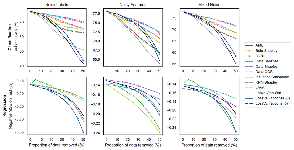
The experimental setup for the point removal experiment (graphic below) is similar. However, here the goal is to remove the highest valued data points from the training set and see how a model trained on this training set performs. This means, that a better Data Valuation method will lead to a faster degradation in model performance because it removes important data points earlier. We found that LossVal matches state-of-the-art methods.

For more detailed results, take a look at our paper.
Conclusion
The idea behind LossVal is simple: Use the gradient descent to find an optimal weight for each data point. The weight signifies the importance of the data point.
Our experiments show that LossVal achieves state-of-the-art performance on the OpenDataVal benchmark. LossVal has a lower time complexity than all other model-based approaches we tested and demonstrates a more robust performance over different types of noise and tasks.
Overall, LossVal presents a efficient alternative to other state-of-the-art Data Valuation approaches for neural networks.
Feel free to get in touch via LinkedIn
LossVal Explained: Efficiently Estimate the Importance of Your Training Data was originally published in Towards Data Science on Medium, where people are continuing the conversation by highlighting and responding to this story.
LossVal Explained: Efficient Data Valuation for Neural NetworksHow to exploit the loss function to efficiently estimate the importance of your training dataData Valuation visualized. Understanding how important each training sample is for the performance of your machine learning model. (Image by author.)This blog post summarizes and explains our paper “LossVal: Efficient Data Valuation for Neural Networks”.Not all data is created equal: Some training data points influence the training of a machine learning model much more than others. Understanding the influence of each data point is often highly inefficient and often relies on repeated retraining of the model. LossVal presents a new approach to this, that efficiently integrates the Data Valuation process into the loss function of an artificial neural network.What is Data Valuation?Machine Learning models are often trained with large datasets. In most cases, not all training samples in such a dataset are equally helpful or informative for the model. For example, if a data point is noisy or has a wrong label, it is less informative for your machine learning model. For one of the tasks in our paper, we trained a machine-learning model on a vehicle crash test dataset to predict how harmful a crash would be for an occupant, based on some vehicle parameters. Some of the data points are from cars of the 80s and 90s! You can imagine, that very old cars may be less important for the model’s predictions on modern cars.The process of understanding the effect of each training sample on the machine-learning model is called Data Valuation, where an importance score is assigned to each training sample. Data Valuation is a growing field connected to data markets, explainable AI, active learning, and many more. Many approaches have been proposed, like Data Shapley, Influence Functions, or LAVA. To learn more about this, you can check out my recent blog post that presents different Data Valuation methods and applications.LossValThe basic idea behind LossVal is to “learn” the importance score of each sample while training the model, similar to how the model weights are learned. This saves us from rerunning the training of the model multiple times and from having to track all model weight updates during the training.To achieve this, we can modify standard loss functions like means squared error (MSE) and cross-entropy loss. We incorporate instance-based weights into the loss and multiply it by a weighted distance function. In general, the LossVal loss functions have the following form:https://medium.com/media/b2524fa59ac79e1633ebd65045e6bca4/hrefwhere ℒ indicates the weighted target loss (weighted MSE or cross-entropy) and OT indicates a weighted distribution distance (OT stands for optimal transport). This results in new loss functions that can be used like any other loss function for training a neural network. However, during each training step, the weights w in the loss are updated using the gradient descent.We demonstrate this for regression tasks using the MSE and for classification using the cross-entropy loss. Afterward, we take a closer look at the distribution distance OT.LossVal for RegressionLet’s start with the MSE. The standard MSE is the squared difference between the model prediction ŷ and the correct prediction y (with n being the index of the training sample):https://medium.com/media/a5ae23d613cad57cebf9edf35066a2fd/hrefFor LossVal, we modify the MSE in two steps: First, a weight wₙ is included for each training instance n. Second, the whole MSE is multiplied with a weighted distribution distance function.https://medium.com/media/f99d0bf5c6397a1413af6e7c0cd1bbc2/hrefLossVal for ClassificationThe cross-entropy loss is typically expressed like this:https://medium.com/media/afea75b0dea4cc524a32636c32013d1d/hrefWe can modify the cross-entropy loss in the same way as the MSE:https://medium.com/media/6a02a1027b1f9d2dc2b2adb276534e71/hrefThe Optimal Transport DistanceThe optimal transport distance is the minimum effort you need to transform one distribution into another. It is also known as the earth mover distance, coming from the analogy of the fastest way to fill a hole with a pile of dirt. OT can be defined as:https://medium.com/media/db5f30eeb15fc7b2d6fbd4340909d5da/hrefwhere c is the cost of moving point xₙ to xⱼ. Each γ is a possible transport plan, defining how the points are moved. The optimal transport plan is the γ* with the least effort involved (the smallest distribution distance). Note that we include the weights w in the cost function via joint distribution Π(w, 1). In other words, OTᵥᵥ is the weighted distance between the training and the validation set. You can find an in-depth explanation for optimal transport here.In a more practical sense, minimizing OTᵥᵥ by changing the weights will assign higher weights to the training data points similar to the validation data. Effectively, noisy samples get a smaller weight.ImplementationOur implementation and all data are available on GitHub. The code below shows the implementation of LossVal for the mean squared error.def LossVal_mse(train_X: torch.Tensor, train_y_true: torch.Tensor, train_y_pred: torch.Tensor, val_X: torch.Tensor, sample_ids: torch.Tensor weights: torch.Tensor, device: torch.device) -> torch.Tensor: weights = weights.index_select(0, sample_ids) # Select the weights corresponding to the sample_ids # Step 1: Compute the weighted mse loss loss = torch.sum((train_y_true – train_y_pred) ** 2, dim=1) weighted_loss = torch.sum(weights @ loss) # Loss is a vector, weights is a matrix # Step 2: Compute the Sinkhorn distance between the training and validation distributions sinkhorn_distance = SamplesLoss(loss=”sinkhorn”) dist_loss = sinkhorn_distance(weights, train_X, torch.ones(val_X.shape[0], requires_grad=True).to(device), val_X) # Step 3: Combine mse and Sinkhorn distance return weighted_loss * dist_loss**2This loss function works like any other loss function in pytorch, with some peculiarities: the parameters include the validation set, sample weights, and the indices of the samples in the batch. This is necessary to select the correct weights for the batched samples for calculating the weighted loss. Keep in mind that this implementation relies on the automatic gradient calculation of pytorch. That means the sample weights vector needs to be part of the model parameters. This way, the optimization of the weights profits from the optimizer implementation, like Adam. Alternatively, one could also update the weights per hand, using the gradient of the loss with respect to each weight i. The implementation for cross-entropy works equivalently, but you need to replace line 8.But does it work?Benchmark comparison of different Data Valuation methods for noisy sample detection. Higher is better. (Image by author.)The graphic above shows the comparison between different Data Valuation approaches on the noisy sample detection task. This task is defined by the OpenDataVal benchmark. First, noise is added to p% of the training data, then the Data Valuation is used to find the noisy samples. Better methods will find more of the noisy samples, hence achieving a higher F1 score. The graph above shows the average over 6 datasets for classification and 6 datasets for regression. We tested 3 different noise types; noisy labels, noisy features, and mixed noise. In the mixed noise condition, half of the noisy sample have feature noise and the other half have label noise. In noisy sample detection, LossVal outperforms all other methods for label noise and mixed noise. However, LAVA performs better for feature noise.The experimental setup for the point removal experiment (graphic below) is similar. However, here the goal is to remove the highest valued data points from the training set and see how a model trained on this training set performs. This means, that a better Data Valuation method will lead to a faster degradation in model performance because it removes important data points earlier. We found that LossVal matches state-of-the-art methods.Benchmark comparison of different Data Valuation methods for removal of high-value points. Lower is better. (Image by author.)For more detailed results, take a look at our paper.ConclusionThe idea behind LossVal is simple: Use the gradient descent to find an optimal weight for each data point. The weight signifies the importance of the data point.Our experiments show that LossVal achieves state-of-the-art performance on the OpenDataVal benchmark. LossVal has a lower time complexity than all other model-based approaches we tested and demonstrates a more robust performance over different types of noise and tasks.Overall, LossVal presents a efficient alternative to other state-of-the-art Data Valuation approaches for neural networks.Feel free to get in touch via LinkedInLossVal Explained: Efficiently Estimate the Importance of Your Training Data was originally published in Towards Data Science on Medium, where people are continuing the conversation by highlighting and responding to this story. data-science, data-valuation, thoughts-and-theory, machine-learning, deep-learning Towards Data Science – MediumRead More

 Add to favorites


0 Comments