Speeding up Llama: A hybrid approach to attention mechanisms

In this article, we will see how to replace softmax self-attention in Llama-3.2-1B with hybrid attention combining softmax sliding window and linear attention. This implementation will help us better understand the growing interest in linear attention research, while also examining its limitations and potential future directions.
This walkthrough builds upon the following works:
- LoLCATs: On Low-Rank Linearizing of Large Language Models
- An Empirical Study of Mamba-based Language Models
- Linearizing Attention
This article will be mostly a recreation of the LoLCATs paper using Llama 3.2 1B, where we will replace 50% of self-attention layers in a pretrained Llama model. The article consists of four main parts:
- Hybrid Attention Block
- Attention Transfer
- LoRA finetuning
- Evaluation
The main goal of this article is that can we somehow replace softmax attention in already trained models so that we can speed up inference while not losing too much on accuracy. If we can achieve this then we can bring the cost of using LLMs down drastically!
LlamaSdpAttention
Let’s see what the Llama-3.2-1B model looks like:
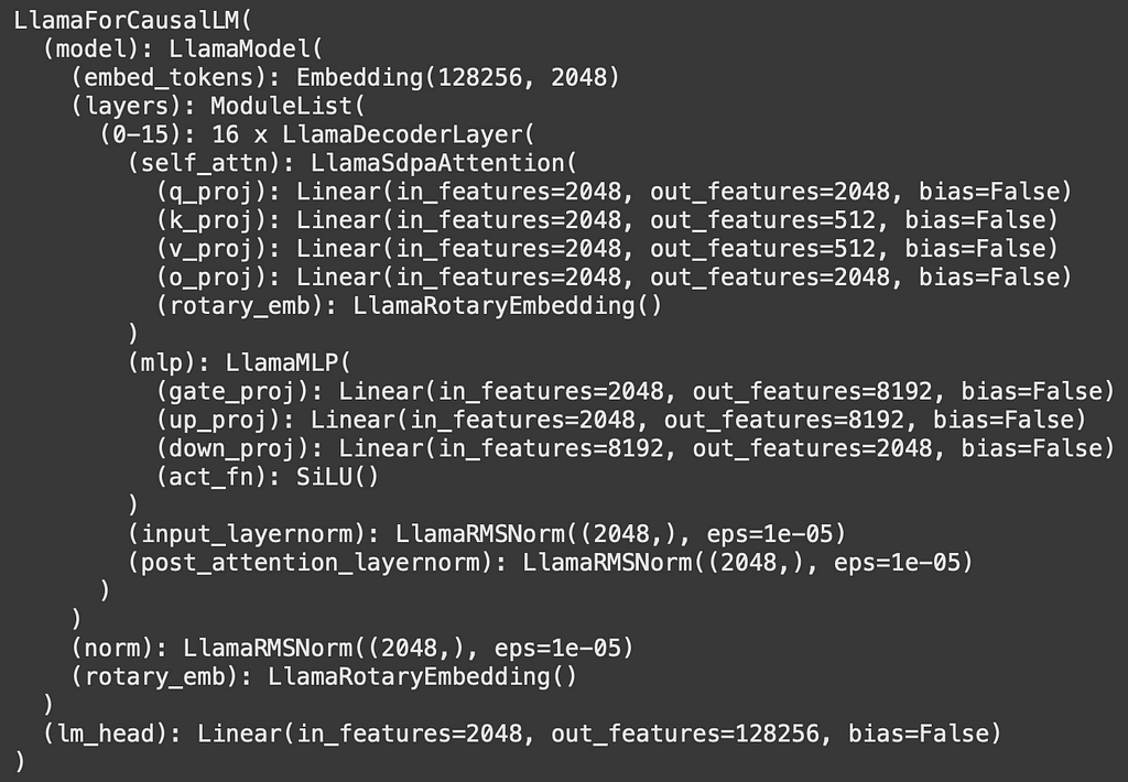
As we can see we have 16 repeating decoder blocks, our focus will be on the self_attn part so the goal of this section is to understand how the LlamaSdpAttention block works! Let’s see what the definition of LlamaSdpAttention is:
class LlamaSdpaAttention(LlamaAttention):
    """
    Llama attention module using torch.nn.functional.scaled_dot_product_attention. This module inherits from
    `LlamaAttention` as the weights of the module stays untouched. The only changes are on the forward pass to adapt to
    SDPA API.
    """
You can check what this function looks like using the following code:
import inspect

attention_layer = model.model.layers[0].self_attn
print(inspect.getsource(attention_layer.__class__))
Let’s go over the main parts of this code and understand what each part is doing and see where we need to make a change,
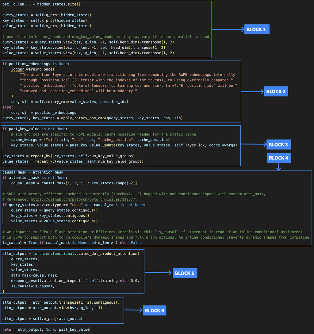
Let’s take a dummy input to be of the shape [2,4,2048] → [batch_size, seq_len, embedding dimension]. Llama uses multi-headed attn with 32 heads.
Block 1:
After proj → query_states is a tensor of [2,4,2048], key_states is a tensor of [2,4,512] and value_states is a tensor of [2,4,512].
After view and transpose it is: query_states → [2,32,4,64] key_states → [2,8,4,64] value_states → [2,8,4,64]
Here 64 is the embedding dimension, key and value have heads as 8 because llama uses key-value groups where basically out of the 32 total heads, groups of 4 heads share the same key_states and value_states among the 32 total heads.
Block 2:
In this block we just apply positional encoding in particular llama uses Rotary Position Embeddings (RoPE). I won’t go into detail why this is needed but you can read the following article to get a better idea:
Master Positional Encoding: Part I
Block 3:
Here we just apply the repeat_kv function which just repeats the kv value in the groups of 4, also we use past_key_value so that we can use some precomputed kv values so that we don’t have to compute them again for computational efficiency.
Block 4:
Block 4 handles two main preparation steps for attention: setting up the causal mask to ensure tokens only attend to previous positions, and optimizing memory layout with contiguous tensors for efficient GPU operations.
Block 5:
This is where we apply softmax attention — the component we’ll be replacing in our implementation.
Block 6:
The attention output will be a tensor of shape [2, 32, 4, 64]. We convert it back to [2, 4, 2048] and apply the final output projection.
And that’s the journey of an input through Llama self-attention!
Hybrid Attention Block
So now let’s look at our HybridAttention block:
class HybridAttention(LlamaSdpaAttention):
    def __init__(self, config, layer_idx=None):
        super().__init__(config, layer_idx=layer_idx)
        self.window_size = 64
        #self.layer_idx = layer_idx

        # Initialize learnable factors
        # Create one factor pair per attention head
        num_heads = config.num_attention_heads
        self.window_factors = torch.nn.Parameter(torch.ones(1, num_heads, 1, 1) * 0.5)
        self.linear_factors = torch.nn.Parameter(torch.ones(1, num_heads, 1, 1) * 0.5)

        self.factor_activation = torch.nn.Sigmoid()

    def sliding_window_attention(self, query_states, key_states, value_states, window_size, window_factor):
        """Compute sliding window attention"""
        batch_size, num_heads, seq_len, head_dim = query_states.shape

        key_windows = F.pad(key_states, (0, 0, window_size - 1, 0), value=0)
        key_windows = key_windows.unfold(2, window_size, 1)

        value_windows = F.pad(value_states, (0, 0, window_size - 1, 0), value=0)
        value_windows = value_windows.unfold(2, window_size, 1)

        attn_weights = torch.einsum('bhld,bhldw->bhlw', query_states, key_windows) * (head_dim ** -0.5)
        attn_weights = torch.where(attn_weights == 0,
                                 torch.tensor(-float('inf'), device=attn_weights.device),
                                 attn_weights)

        # Apply learnable window factor (with sigmoid to ensure positivity)
        attn_weights = self.factor_activation(window_factor) * F.softmax(attn_weights, dim=-1)

        attn_output = torch.einsum('bhlw,bhldw->bhld', attn_weights, value_windows)
        sum_weights = attn_weights.sum(dim=-1, keepdim=True)

        return attn_output, sum_weights

    def linear_attention(self, query_states, key_states, value_states, window_size, linear_factor):
        """Compute linear attention with cumsum"""
        def feature_map(x):
            return F.elu(x) + 1

        query_prime = feature_map(query_states)
        key_prime = feature_map(key_states)

        key_prime = F.pad(key_prime, (0, 0, window_size, 0), value=0)[:, :, :-window_size, :]
        value_padded = F.pad(value_states, (0, 0, window_size, 0), value=0)[:, :, :-window_size, :]

        # Compute KV
        kv = torch.einsum('bhlf,bhld->bhlfd', key_prime, value_padded)
        # Apply learnable linear factor (with sigmoid to ensure positivity)
        qkv = self.factor_activation(linear_factor) * torch.einsum('bhlf,bhlfd->bhld',
                                                                  query_prime,
                                                                  kv.cumsum(dim=2))

        sum_k = key_prime.cumsum(dim=2)
        sum_qk = self.factor_activation(linear_factor) * torch.einsum('bhld,bhld->bhl',
                                                                     query_prime,
                                                                     sum_k)[..., None]
        sum_qk = torch.where(sum_qk == 0, torch.tensor(1e-12, device=sum_qk.device), sum_qk)

        return qkv, sum_qk

    def hybrid_attention(self, query_states, key_states, value_states):
        """Combine sliding window and linear attention with learnable factors"""
        qkv_window, sum_window = self.sliding_window_attention(
            query_states, key_states, value_states,
            self.window_size, self.window_factors
        )

        qkv_linear, sum_linear = self.linear_attention(
            query_states, key_states, value_states,
            self.window_size, self.linear_factors
        )

        output = (qkv_window + qkv_linear) / (sum_window + sum_linear)
        return output

    def forward(
        self,
        hidden_states: torch.Tensor,
        attention_mask: Optional[torch.Tensor] = None,
        position_ids: Optional[torch.LongTensor] = None,
        past_key_value: Optional[Cache] = None,
        output_attentions: bool = False,
        use_cache: bool = False,
        cache_position: Optional[torch.LongTensor] = None,
        position_embeddings: Optional[Tuple[torch.Tensor, torch.Tensor]] = None,
        **kwargs,
    ):
        bsz, q_len, _ = hidden_states.size()

        query_states = self.q_proj(hidden_states)
        key_states = self.k_proj(hidden_states)
        value_states = self.v_proj(hidden_states)

        query_states = query_states.view(bsz, q_len, -1, self.head_dim).transpose(1, 2)
        key_states = key_states.view(bsz, q_len, -1, self.head_dim).transpose(1, 2)
        value_states = value_states.view(bsz, q_len, -1, self.head_dim).transpose(1, 2)

        if position_embeddings is None:
            cos, sin = self.rotary_emb(value_states, position_ids)
        else:
            cos, sin = position_embeddings
        query_states, key_states = apply_rotary_pos_emb(query_states, key_states, cos, sin)

        if past_key_value is not None:
            cache_kwargs = {"sin": sin, "cos": cos, "cache_position": cache_position}
            key_states, value_states = past_key_value.update(key_states, value_states, self.layer_idx, cache_kwargs)

        key_states = repeat_kv(key_states, self.num_key_value_groups)
        value_states = repeat_kv(value_states, self.num_key_value_groups)

        attn_output = self.hybrid_attention(
            query_states,
            key_states,
            value_states
        )

        attn_output = attn_output.transpose(1, 2).contiguous()
        attn_output = attn_output.view(bsz, q_len, -1)
        attn_output = self.o_proj(attn_output)

        return attn_output, None, past_key_value
We only made one change in forward(), we replaced block 5 with the following:
attn_output = self.hybrid_attention(
            query_states,
            key_states,
            value_states
        )
We basically partitioned the attention mechanism into sliding window and linear attention blocks.
Sliding Window Attention:
def sliding_window_attention(self, query_states, key_states, value_states, window_size, window_factor):
        """Compute sliding window attention"""
        batch_size, num_heads, seq_len, head_dim = query_states.shape

        key_windows = F.pad(key_states, (0, 0, window_size - 1, 0), value=0)
        key_windows = key_windows.unfold(2, window_size, 1)

        value_windows = F.pad(value_states, (0, 0, window_size - 1, 0), value=0)
        value_windows = value_windows.unfold(2, window_size, 1)

        attn_weights = torch.einsum('bhld,bhldw->bhlw', query_states, key_windows) * (head_dim ** -0.5)
        attn_weights = torch.where(attn_weights == 0,
                                 torch.tensor(-float('inf'), device=attn_weights.device),
                                 attn_weights)

        # Apply learnable window factor (with sigmoid to ensure positivity)
        attn_weights = self.factor_activation(window_factor) * F.softmax(attn_weights, dim=-1)

        attn_output = torch.einsum('bhlw,bhldw->bhld', attn_weights, value_windows)
        sum_weights = attn_weights.sum(dim=-1, keepdim=True)

        return attn_output, sum_weights
For a deeper understanding of window attention concepts, I recommend referring to this paper:
Efficient Streaming Language Models with Attention Sinks
The idea I have implemented here is that instead of calculating the attention of all key-value pairs together(where each token attends to every other token), we break it into windows of ‘w’ size and then calculate the attention for each window. Using this in the above code, the time complexity comes down from O(n²) to O(n*w), since each token only needs to attend to w tokens instead of all n tokens. It can be made even better by using concepts such as sinks and only doing window for last w tokens which I might implement in future updates.
Linear Attention:
def linear_attention(self, query_states, key_states, value_states, window_size, linear_factor):
        """Compute linear attention with cumsum"""
        def feature_map(x):
            return F.elu(x) + 1

        query_prime = feature_map(query_states)
        key_prime = feature_map(key_states)

        key_prime = F.pad(key_prime, (0, 0, window_size, 0), value=0)[:, :, :-window_size, :]
        value_padded = F.pad(value_states, (0, 0, window_size, 0), value=0)[:, :, :-window_size, :]

        # Compute KV
        kv = torch.einsum('bhlf,bhld->bhlfd', key_prime, value_padded)
        # Apply learnable linear factor (with sigmoid to ensure positivity)
        qkv = self.factor_activation(linear_factor) * torch.einsum('bhlf,bhlfd->bhld',
                                                                  query_prime,
                                                                  kv.cumsum(dim=2))

        sum_k = key_prime.cumsum(dim=2)
        sum_qk = self.factor_activation(linear_factor) * torch.einsum('bhld,bhld->bhl',
                                                                     query_prime,
                                                                     sum_k)[..., None]
        sum_qk = torch.where(sum_qk == 0, torch.tensor(1e-12, device=sum_qk.device), sum_qk)

        return qkv, sum_qk
For linear attention, I use a very simple feature map of elu(x) + 1 but the main part to note there is the initial padding being done. The idea here is that we can use linear attention only for the first [sequence length — window size] as we already have sliding window to keep track of recent context.
The combination of these two types of attention becomes our new hybrid attention and we use window_factor and linear_factor as learnable parameters that control how much each type of attention contributes to the final output.
Now that we have our hybrid block, taking inspiration from the “An Empirical Study of Mamba-based Language Models” paper, we will replace only half the softmax attention layers that too in an alternate order. Llama-3.2-1B has 16 softmax attention layers and we shall replace 8 of those in the order: [0,2,4,6,8,10,12,14].
Attention Transfer
The implementation follows the methodology described in “LoLCATs: On Low-Rank Linearizing of Large Language Models”. The attention transfer step involves initializing 8 hybrid blocks with the weights from the original blocks and for training I used 1M tokens from the 10B version of fineweb-edu[1].
The basic goal here is that, we will freeze all the parameters in llama-3.2–1B and then do a forward pass with one train input. Using this we can get the input and output of each of our self attention blocks. We can then pass this same input from the corresponding hybrid block and then take the MSE loss between the two and train the hybrid blocks. What this helps us do is to explicitly tell the hybrid block to mimic the output of softmax attention which will help preserve accuracy. We do this separately for all the blocks and once trained we can replace the the self attention in llama-3.2–1B with our hybrid blocks now. Taking a sample output from this new model looks something like,

The current model outputs lack coherence and meaning — an issue that our next implementation phase will specifically target and resolve.
The code for this step — Llama_attn_transfer.ipynb
LoRA Finetune
I won’t go into the details of LoRA, you could go through the following article if you want to understand LoRA better:
LoRA — Intuitively and Exhaustively Explained
But the main goal with this step is that so far we trained each hybrid block separately to mimic softmax but we still haven’t trained/finetuned the entire model post adding these blocks to actually work together for text generation. So in this step we use the Dolly-15K Dataset[2] which is an instruction tuning dataset to finetune our model for text generation using LoRA and we only finetune the parameters in the hybrid attention blocks while every other parameter is frozen.
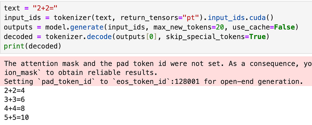
We can clearly see the model is able to generate much better text post this finetuning. Now after attention transfer and finetuning, we have a model we can actually benchmark!
The code for this step — llama_lora_finetune.ipynb
Evaluation
We went through all these steps so now it’s time compare our hybrid model with the original Llama-3.2-1B. Our main expectations are that our model should be faster during inference while its accuracy should remain reasonably close to that of Llama-3.2-1B.
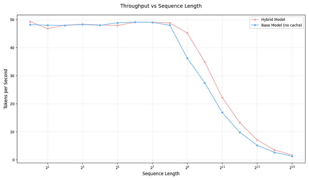
Evaluating both models on throughput for sequence-lengths ranging from 2⁰ to 2¹⁵, we can see that initially both models are pretty close in performance. However, as the sequence length increases, the hybrid model becomes notably faster than the base model — matching our expectations. It’s important to note that these tokens/sec measurements vary significantly depending on the GPU used.
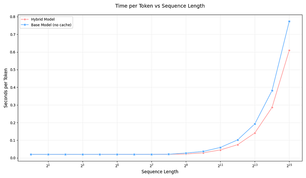
Looking at seconds taken per token, we see a similar pattern: initially, both models have nearly the same speed, but as the sequence length increases, we observe the computational advantages that linear + sliding window attention brings.
☑️ We meet our first expectation that our hybrid is faster than llama-3.2-1B.
Now let’s look at accuracy, For this, I benchmarked the models on MMLU[3] where each model had to answer multiple-choice questions with 4 options. The model’s prediction is determined by examining the logits it assigns to tokens [‘A’, ‘B’, ‘C’, ‘D’], with the highest logit indicating the predicted answer.
╔═════════════════════════╦══════════╦═══════════╦════════════════════╗
║          Model          ║ Num Shot ║    GPU    ║ macro_avg/acc_char ║
╠═════════════════════════╬══════════╬═══════════╬════════════════════╣
║ Hybrid                  ║        5 ║ RTX A6000 ║              27.36 ║
║ Llama 3.2 1B (No Cache) ║        5 ║ RTX A6000 ║              25.38 ║
║ Llama 3.2 1B (No Cache) ║        5 ║ L40S      ║              32.13 ║
║ Hybrid                  ║        0 ║ RTX A6000 ║              27.26 ║
║ Llama 3.2 1B (No Cache) ║        0 ║ RTX A6000 ║              25.50 ║
╚═════════════════════════╩══════════╩═══════════╩════════════════════╝
The test results reveal an intriguing insight into model evaluation. While the Hybrid model slightly outperforms Llama-3.2-1B, this difference (approximately 2%) should be considered insignificant, especially given that the Hybrid model underwent additional training, particularly with instruction tuning datasets.
The most fascinating observation is the substantial performance variance when running identical code on different GPUs. When Llama-3.2-1B was run on an L40S GPU versus an RTX A6000, the accuracy jumped from 25.38% to 32.13% — a significant difference considering all other variables remained constant. This difference comes down to how different GPUs handle floating-point operations, which shows just how much hardware choices can unexpectedly affect your model’s performance.
Another striking finding is the lack of difference between 5-shot and 0-shot performance in these results, particularly on the RTX A6000. This is unexpected, as 5-shot prompting typically improves performance, especially for base models like Llama-3.2-1B. In fact, when running the Llama-3.2-1B on the L40S GPU, I have observed a notable gap between 5-shot and 0-shot scores — again highlighting how GPU differences can affect benchmark scores.
It would be a fun future exercise to benchmark the same model with all the same variables but with different GPUs.
- MMLU 0-shot evaluation code — MMLU_eval-0shot.ipynb
- MMLU 5-shot evaluation code — MMLU_eval-5shot.ipynb
- Inference speed evaluation code — Linear_llama_eval_inference_speed.ipynb
Conclusion
I hope this article has demonstrated both the potential of softmax attention alternatives and the inherent strengths of traditional softmax attention. Using relatively modest computational resources and a small dataset, we were able to achieve faster inference speeds while maintaining comparable accuracy levels with our hybrid approach.
Another point to understand is that softmax based attention transformers have gone through a lot of hardware optimizations which make them competitive with linear alternatives when it comes to computational complexity, if the same effort is put into architectures like mamba maybe they can be more competitive then.
A promising approach is using a hybrid of softmax attention and linear attention alternatives to try to get the best of both worlds. Nvidia did this in “An Empirical Study of Mamba-based Language Models” and showed how a hybrid approach is an effective alternative.
Hopefully you all learnt something from this article!
All the code for this can be found at — Linearizing-Llama-3.2–1B
Acknowledgment
This blog post was inspired by coursework from my graduate studies during Fall 2024 at University of Michigan. While the courses provided the foundational knowledge and motivation to explore these topics, any errors or misinterpretations in this article are entirely my own. This represents my personal understanding and exploration of the material.
License References
[1] — fineweb-edu: The dataset is released under the Open Data Commons Attribution License (ODC-By) v1.0 license.
[2] — Dolly-15K: The dataset is subject to CC BY-SA 3.0 license.
[3] — MMLU: MIT license
Linearizing Llama was originally published in Towards Data Science on Medium, where people are continuing the conversation by highlighting and responding to this story.
Speeding up Llama: A hybrid approach to attention mechanismsSource: Image by Author (Generated using Gemini 1.5 Flash)In this article, we will see how to replace softmax self-attention in Llama-3.2-1B with hybrid attention combining softmax sliding window and linear attention. This implementation will help us better understand the growing interest in linear attention research, while also examining its limitations and potential future directions.This walkthrough builds upon the following works:LoLCATs: On Low-Rank Linearizing of Large Language ModelsAn Empirical Study of Mamba-based Language ModelsLinearizing AttentionThis article will be mostly a recreation of the LoLCATs paper using Llama 3.2 1B, where we will replace 50% of self-attention layers in a pretrained Llama model. The article consists of four main parts:Hybrid Attention BlockAttention TransferLoRA finetuningEvaluationThe main goal of this article is that can we somehow replace softmax attention in already trained models so that we can speed up inference while not losing too much on accuracy. If we can achieve this then we can bring the cost of using LLMs down drastically!LlamaSdpAttentionLet’s see what the Llama-3.2-1B model looks like:Source: Image by AuthorAs we can see we have 16 repeating decoder blocks, our focus will be on the self_attn part so the goal of this section is to understand how the LlamaSdpAttention block works! Let’s see what the definition of LlamaSdpAttention is:class LlamaSdpaAttention(LlamaAttention): “”” Llama attention module using torch.nn.functional.scaled_dot_product_attention. This module inherits from `LlamaAttention` as the weights of the module stays untouched. The only changes are on the forward pass to adapt to SDPA API. “””You can check what this function looks like using the following code:import inspectattention_layer = model.model.layers[0].self_attnprint(inspect.getsource(attention_layer.__class__))Let’s go over the main parts of this code and understand what each part is doing and see where we need to make a change,Source: Image by AuthorLet’s take a dummy input to be of the shape [2,4,2048] → [batch_size, seq_len, embedding dimension]. Llama uses multi-headed attn with 32 heads.Block 1:After proj → query_states is a tensor of [2,4,2048], key_states is a tensor of [2,4,512] and value_states is a tensor of [2,4,512].After view and transpose it is: query_states → [2,32,4,64] key_states → [2,8,4,64] value_states → [2,8,4,64]Here 64 is the embedding dimension, key and value have heads as 8 because llama uses key-value groups where basically out of the 32 total heads, groups of 4 heads share the same key_states and value_states among the 32 total heads.Block 2:In this block we just apply positional encoding in particular llama uses Rotary Position Embeddings (RoPE). I won’t go into detail why this is needed but you can read the following article to get a better idea:Master Positional Encoding: Part IBlock 3:Here we just apply the repeat_kv function which just repeats the kv value in the groups of 4, also we use past_key_value so that we can use some precomputed kv values so that we don’t have to compute them again for computational efficiency.Block 4:Block 4 handles two main preparation steps for attention: setting up the causal mask to ensure tokens only attend to previous positions, and optimizing memory layout with contiguous tensors for efficient GPU operations.Block 5:This is where we apply softmax attention — the component we’ll be replacing in our implementation.Block 6:The attention output will be a tensor of shape [2, 32, 4, 64]. We convert it back to [2, 4, 2048] and apply the final output projection.And that’s the journey of an input through Llama self-attention!Hybrid Attention BlockSo now let’s look at our HybridAttention block:class HybridAttention(LlamaSdpaAttention): def __init__(self, config, layer_idx=None): super().__init__(config, layer_idx=layer_idx) self.window_size = 64 #self.layer_idx = layer_idx # Initialize learnable factors # Create one factor pair per attention head num_heads = config.num_attention_heads self.window_factors = torch.nn.Parameter(torch.ones(1, num_heads, 1, 1) * 0.5) self.linear_factors = torch.nn.Parameter(torch.ones(1, num_heads, 1, 1) * 0.5) self.factor_activation = torch.nn.Sigmoid() def sliding_window_attention(self, query_states, key_states, value_states, window_size, window_factor): “””Compute sliding window attention””” batch_size, num_heads, seq_len, head_dim = query_states.shape key_windows = F.pad(key_states, (0, 0, window_size – 1, 0), value=0) key_windows = key_windows.unfold(2, window_size, 1) value_windows = F.pad(value_states, (0, 0, window_size – 1, 0), value=0) value_windows = value_windows.unfold(2, window_size, 1) attn_weights = torch.einsum(‘bhld,bhldw->bhlw’, query_states, key_windows) * (head_dim ** -0.5) attn_weights = torch.where(attn_weights == 0, torch.tensor(-float(‘inf’), device=attn_weights.device), attn_weights) # Apply learnable window factor (with sigmoid to ensure positivity) attn_weights = self.factor_activation(window_factor) * F.softmax(attn_weights, dim=-1) attn_output = torch.einsum(‘bhlw,bhldw->bhld’, attn_weights, value_windows) sum_weights = attn_weights.sum(dim=-1, keepdim=True) return attn_output, sum_weights def linear_attention(self, query_states, key_states, value_states, window_size, linear_factor): “””Compute linear attention with cumsum””” def feature_map(x): return F.elu(x) + 1 query_prime = feature_map(query_states) key_prime = feature_map(key_states) key_prime = F.pad(key_prime, (0, 0, window_size, 0), value=0)[:, :, :-window_size, :] value_padded = F.pad(value_states, (0, 0, window_size, 0), value=0)[:, :, :-window_size, :] # Compute KV kv = torch.einsum(‘bhlf,bhld->bhlfd’, key_prime, value_padded) # Apply learnable linear factor (with sigmoid to ensure positivity) qkv = self.factor_activation(linear_factor) * torch.einsum(‘bhlf,bhlfd->bhld’, query_prime, kv.cumsum(dim=2)) sum_k = key_prime.cumsum(dim=2) sum_qk = self.factor_activation(linear_factor) * torch.einsum(‘bhld,bhld->bhl’, query_prime, sum_k)[…, None] sum_qk = torch.where(sum_qk == 0, torch.tensor(1e-12, device=sum_qk.device), sum_qk) return qkv, sum_qk def hybrid_attention(self, query_states, key_states, value_states): “””Combine sliding window and linear attention with learnable factors””” qkv_window, sum_window = self.sliding_window_attention( query_states, key_states, value_states, self.window_size, self.window_factors ) qkv_linear, sum_linear = self.linear_attention( query_states, key_states, value_states, self.window_size, self.linear_factors ) output = (qkv_window + qkv_linear) / (sum_window + sum_linear) return output def forward( self, hidden_states: torch.Tensor, attention_mask: Optional[torch.Tensor] = None, position_ids: Optional[torch.LongTensor] = None, past_key_value: Optional[Cache] = None, output_attentions: bool = False, use_cache: bool = False, cache_position: Optional[torch.LongTensor] = None, position_embeddings: Optional[Tuple[torch.Tensor, torch.Tensor]] = None, **kwargs, ): bsz, q_len, _ = hidden_states.size() query_states = self.q_proj(hidden_states) key_states = self.k_proj(hidden_states) value_states = self.v_proj(hidden_states) query_states = query_states.view(bsz, q_len, -1, self.head_dim).transpose(1, 2) key_states = key_states.view(bsz, q_len, -1, self.head_dim).transpose(1, 2) value_states = value_states.view(bsz, q_len, -1, self.head_dim).transpose(1, 2) if position_embeddings is None: cos, sin = self.rotary_emb(value_states, position_ids) else: cos, sin = position_embeddings query_states, key_states = apply_rotary_pos_emb(query_states, key_states, cos, sin) if past_key_value is not None: cache_kwargs = {“sin”: sin, “cos”: cos, “cache_position”: cache_position} key_states, value_states = past_key_value.update(key_states, value_states, self.layer_idx, cache_kwargs) key_states = repeat_kv(key_states, self.num_key_value_groups) value_states = repeat_kv(value_states, self.num_key_value_groups) attn_output = self.hybrid_attention( query_states, key_states, value_states ) attn_output = attn_output.transpose(1, 2).contiguous() attn_output = attn_output.view(bsz, q_len, -1) attn_output = self.o_proj(attn_output) return attn_output, None, past_key_valueWe only made one change in forward(), we replaced block 5 with the following:attn_output = self.hybrid_attention( query_states, key_states, value_states )We basically partitioned the attention mechanism into sliding window and linear attention blocks.Sliding Window Attention:def sliding_window_attention(self, query_states, key_states, value_states, window_size, window_factor): “””Compute sliding window attention””” batch_size, num_heads, seq_len, head_dim = query_states.shape key_windows = F.pad(key_states, (0, 0, window_size – 1, 0), value=0) key_windows = key_windows.unfold(2, window_size, 1) value_windows = F.pad(value_states, (0, 0, window_size – 1, 0), value=0) value_windows = value_windows.unfold(2, window_size, 1) attn_weights = torch.einsum(‘bhld,bhldw->bhlw’, query_states, key_windows) * (head_dim ** -0.5) attn_weights = torch.where(attn_weights == 0, torch.tensor(-float(‘inf’), device=attn_weights.device), attn_weights) # Apply learnable window factor (with sigmoid to ensure positivity) attn_weights = self.factor_activation(window_factor) * F.softmax(attn_weights, dim=-1) attn_output = torch.einsum(‘bhlw,bhldw->bhld’, attn_weights, value_windows) sum_weights = attn_weights.sum(dim=-1, keepdim=True) return attn_output, sum_weightsFor a deeper understanding of window attention concepts, I recommend referring to this paper:Efficient Streaming Language Models with Attention SinksThe idea I have implemented here is that instead of calculating the attention of all key-value pairs together(where each token attends to every other token), we break it into windows of ‘w’ size and then calculate the attention for each window. Using this in the above code, the time complexity comes down from O(n²) to O(n*w), since each token only needs to attend to w tokens instead of all n tokens. It can be made even better by using concepts such as sinks and only doing window for last w tokens which I might implement in future updates.Linear Attention:def linear_attention(self, query_states, key_states, value_states, window_size, linear_factor): “””Compute linear attention with cumsum””” def feature_map(x): return F.elu(x) + 1 query_prime = feature_map(query_states) key_prime = feature_map(key_states) key_prime = F.pad(key_prime, (0, 0, window_size, 0), value=0)[:, :, :-window_size, :] value_padded = F.pad(value_states, (0, 0, window_size, 0), value=0)[:, :, :-window_size, :] # Compute KV kv = torch.einsum(‘bhlf,bhld->bhlfd’, key_prime, value_padded) # Apply learnable linear factor (with sigmoid to ensure positivity) qkv = self.factor_activation(linear_factor) * torch.einsum(‘bhlf,bhlfd->bhld’, query_prime, kv.cumsum(dim=2)) sum_k = key_prime.cumsum(dim=2) sum_qk = self.factor_activation(linear_factor) * torch.einsum(‘bhld,bhld->bhl’, query_prime, sum_k)[…, None] sum_qk = torch.where(sum_qk == 0, torch.tensor(1e-12, device=sum_qk.device), sum_qk) return qkv, sum_qkFor linear attention, I use a very simple feature map of elu(x) + 1 but the main part to note there is the initial padding being done. The idea here is that we can use linear attention only for the first [sequence length — window size] as we already have sliding window to keep track of recent context.The combination of these two types of attention becomes our new hybrid attention and we use window_factor and linear_factor as learnable parameters that control how much each type of attention contributes to the final output.Now that we have our hybrid block, taking inspiration from the “An Empirical Study of Mamba-based Language Models” paper, we will replace only half the softmax attention layers that too in an alternate order. Llama-3.2-1B has 16 softmax attention layers and we shall replace 8 of those in the order: [0,2,4,6,8,10,12,14].Attention TransferThe implementation follows the methodology described in “LoLCATs: On Low-Rank Linearizing of Large Language Models”. The attention transfer step involves initializing 8 hybrid blocks with the weights from the original blocks and for training I used 1M tokens from the 10B version of fineweb-edu[1].The basic goal here is that, we will freeze all the parameters in llama-3.2–1B and then do a forward pass with one train input. Using this we can get the input and output of each of our self attention blocks. We can then pass this same input from the corresponding hybrid block and then take the MSE loss between the two and train the hybrid blocks. What this helps us do is to explicitly tell the hybrid block to mimic the output of softmax attention which will help preserve accuracy. We do this separately for all the blocks and once trained we can replace the the self attention in llama-3.2–1B with our hybrid blocks now. Taking a sample output from this new model looks something like,Source: Image by AuthorThe current model outputs lack coherence and meaning — an issue that our next implementation phase will specifically target and resolve.The code for this step — Llama_attn_transfer.ipynbLoRA FinetuneI won’t go into the details of LoRA, you could go through the following article if you want to understand LoRA better:LoRA — Intuitively and Exhaustively ExplainedBut the main goal with this step is that so far we trained each hybrid block separately to mimic softmax but we still haven’t trained/finetuned the entire model post adding these blocks to actually work together for text generation. So in this step we use the Dolly-15K Dataset[2] which is an instruction tuning dataset to finetune our model for text generation using LoRA and we only finetune the parameters in the hybrid attention blocks while every other parameter is frozen.Source: Image by AuthorWe can clearly see the model is able to generate much better text post this finetuning. Now after attention transfer and finetuning, we have a model we can actually benchmark!The code for this step — llama_lora_finetune.ipynbEvaluationWe went through all these steps so now it’s time compare our hybrid model with the original Llama-3.2-1B. Our main expectations are that our model should be faster during inference while its accuracy should remain reasonably close to that of Llama-3.2-1B.Source: Image by AuthorEvaluating both models on throughput for sequence-lengths ranging from 2⁰ to 2¹⁵, we can see that initially both models are pretty close in performance. However, as the sequence length increases, the hybrid model becomes notably faster than the base model — matching our expectations. It’s important to note that these tokens/sec measurements vary significantly depending on the GPU used.Source: Image by AuthorLooking at seconds taken per token, we see a similar pattern: initially, both models have nearly the same speed, but as the sequence length increases, we observe the computational advantages that linear + sliding window attention brings.☑️ We meet our first expectation that our hybrid is faster than llama-3.2-1B.Now let’s look at accuracy, For this, I benchmarked the models on MMLU[3] where each model had to answer multiple-choice questions with 4 options. The model’s prediction is determined by examining the logits it assigns to tokens [‘A’, ‘B’, ‘C’, ‘D’], with the highest logit indicating the predicted answer.╔═════════════════════════╦══════════╦═══════════╦════════════════════╗║ Model ║ Num Shot ║ GPU ║ macro_avg/acc_char ║╠═════════════════════════╬══════════╬═══════════╬════════════════════╣║ Hybrid ║ 5 ║ RTX A6000 ║ 27.36 ║║ Llama 3.2 1B (No Cache) ║ 5 ║ RTX A6000 ║ 25.38 ║║ Llama 3.2 1B (No Cache) ║ 5 ║ L40S ║ 32.13 ║║ Hybrid ║ 0 ║ RTX A6000 ║ 27.26 ║║ Llama 3.2 1B (No Cache) ║ 0 ║ RTX A6000 ║ 25.50 ║╚═════════════════════════╩══════════╩═══════════╩════════════════════╝The test results reveal an intriguing insight into model evaluation. While the Hybrid model slightly outperforms Llama-3.2-1B, this difference (approximately 2%) should be considered insignificant, especially given that the Hybrid model underwent additional training, particularly with instruction tuning datasets.The most fascinating observation is the substantial performance variance when running identical code on different GPUs. When Llama-3.2-1B was run on an L40S GPU versus an RTX A6000, the accuracy jumped from 25.38% to 32.13% — a significant difference considering all other variables remained constant. This difference comes down to how different GPUs handle floating-point operations, which shows just how much hardware choices can unexpectedly affect your model’s performance.Another striking finding is the lack of difference between 5-shot and 0-shot performance in these results, particularly on the RTX A6000. This is unexpected, as 5-shot prompting typically improves performance, especially for base models like Llama-3.2-1B. In fact, when running the Llama-3.2-1B on the L40S GPU, I have observed a notable gap between 5-shot and 0-shot scores — again highlighting how GPU differences can affect benchmark scores.It would be a fun future exercise to benchmark the same model with all the same variables but with different GPUs.MMLU 0-shot evaluation code — MMLU_eval-0shot.ipynbMMLU 5-shot evaluation code — MMLU_eval-5shot.ipynbInference speed evaluation code — Linear_llama_eval_inference_speed.ipynbConclusionI hope this article has demonstrated both the potential of softmax attention alternatives and the inherent strengths of traditional softmax attention. Using relatively modest computational resources and a small dataset, we were able to achieve faster inference speeds while maintaining comparable accuracy levels with our hybrid approach.Another point to understand is that softmax based attention transformers have gone through a lot of hardware optimizations which make them competitive with linear alternatives when it comes to computational complexity, if the same effort is put into architectures like mamba maybe they can be more competitive then.A promising approach is using a hybrid of softmax attention and linear attention alternatives to try to get the best of both worlds. Nvidia did this in “An Empirical Study of Mamba-based Language Models” and showed how a hybrid approach is an effective alternative.Hopefully you all learnt something from this article!All the code for this can be found at — Linearizing-Llama-3.2–1BAcknowledgmentThis blog post was inspired by coursework from my graduate studies during Fall 2024 at University of Michigan. While the courses provided the foundational knowledge and motivation to explore these topics, any errors or misinterpretations in this article are entirely my own. This represents my personal understanding and exploration of the material.License References[1] — fineweb-edu: The dataset is released under the Open Data Commons Attribution License (ODC-By) v1.0 license.[2] — Dolly-15K: The dataset is subject to CC BY-SA 3.0 license.[3] — MMLU: MIT licenseLinearizing Llama was originally published in Towards Data Science on Medium, where people are continuing the conversation by highlighting and responding to this story. llm, attention, llama-3, nlp, large-language-models Towards Data Science – MediumRead More

 Add to favorites


0 Comments