With the help of an intricate geometric construction, we can prove that instance-wise cost functions quickly drive SVC to infinity.
In the previous article in this series, we examined the concept of strategic VC dimension (SVC) and its connection to the Fundamental Theorem of Strategic Learning. We will make use of both of those in this article, alongside the ideas of achievable labelings and strategic shattering coefficients that we explored in the lead-up to them.
Quantifying the Complexity and Learnability of Strategic Classification Problems
If you haven’t read the first article in this series yet, I encourage you to start from there before moving on to the aforementioned article on SVC:
Extending PAC Learning to a Strategic Classification Setting
With the context from the other articles in this series in place, a basic grasp of set theory and geometry will be all you’ll need to understand the theorem and its proof.
How an Instance-Wise Cost Function Affects SVC: Stating the Theorem
As we saw, SVC can be used as a tool to estimate the expressive power of a hypothesis class within a strategic classification context. Having carefully defined SVC as a generalization of the canonical VC dimension, we understand that the two have much in common. When, though, does SVC diverge from its canonical counterpart? Can we come up with a scenario in which the strategic aspect of a classification problem significantly increases its complexity? It turns out we can, with relative ease: linear classification.
Linear classification involves determining whether a data point should be positively or negatively classified based on a linear function applied to its features. Geometrically, we can imagine a linear classifier inducing a linear decision boundary in d-dimensional real space (ℝᵈ ). Anything on one side of the boundary is positively classified, and anything on the other side is negatively classified. In one-dimensional space, the decision boundary is a threshold (as we saw in the previous article). In two-dimensional space, it’s a line dividing the plane. In general, it’s a hyperplane.
In canonical binary classification, the VC dimension of the hypothesis class comprising all linear classifiers in ℝᵈ is d + 1, which is finite. For example, for d = 2 (linear classifiers in ℝ²), the VC dimension is 3. The Fundamental Theorem of Statistical Learning dictates that canonical linear classification is therefore PAC learnable.⁽¹⁾
Intuitively, we might expect the same conclusion to hold for the strategic analog of the problem. After all, linear classifiers are some of the simplest classifiers there are, and reasoning about them can be rather natural.⁽²⁾
However, that simplicity goes out the window as soon as we throw instance-wise cost functions into the mix. As we will prove:
Given a strategic linear classification problem Sᴛʀᴀᴄ⟨H, R, c⟩, there exists an instance-wise cost function c(z; x) = ℓₓ(z – x) such that SVC(H, R, c) = ∞.
In other words, using the Fundamental Theorem of Strategic Learning, we find that linear classification in a strategic setting equipped with an instance-wise cost function is not generally PAC learnable. Interestingly, it will not be PAC learnable even if we strip away as much complexity as we can. In this case, we will do so by focusing on strategic linear classification on the Cartesian plane ( X ⊆ ℝ²) with the homogeneous preference class (R = { 1 }).
The more general conclusion will follow from the counterexample we will show under those simplifying conditions. If strategic linear classification is not PAC learnable in ℝ², there is no way it could be PAC learnable in any higher dimension. Likewise, every other preference class we laid out in our setup is a strict generalization of the homogeneous preference class. If we could prove PAC learnability for any of those preference classes, we would also be able to do so for the simpler case where R = { 1 }.
From Labelings to Points on the Unit Circle: Proof Setup
Based on the assumptions above, we begin by turning our attention to the special case Sᴛʀᴀᴄ⟨Hₗ, { 1 }, c⟩, with Hₗ being the hypothesis class comprising all linear classifiers in ℝ². We then initialize n two-dimensional feature vectors at the origin: ∀ i ≤ n . xᵢ = (0, 0). Since we’re using the homogeneous preference class, we have that ∀ i ≤ n . rᵢ = 1. The only difference between the data points will be in how our cost function behaves on each of them. This is where the crux of the proof lies, as we will soon see.
Before we discuss the cost function at length, though, we need to geometrize the possible labelings of our unlabeled data points. As we saw last time, a set of n unlabeled data points must have exactly 2ⁿ possible labelings. Representing a set of labelings (n-tuples) geometrically in ℝ² is relatively straightforward: we simply select an arbitrary point for each possible labeling. In particular, we will choose 2ⁿ such representative points on the unit circle, each assigned to a possible labeling. While the particular coordinates of the representative points themselves are unimportant, we do require that each such point be unique. We also require that no two points be origin-symmetric with respect to one another.
We will denote this set of representative points by S. Having selected our representative points, we use them to define the origin-symmetric set S’, i.e., S’ = { (-x, –y) : (x, y) ∈ S }. Note that S and S’ are disjoint (S ∩ S’ = ∅) as a consequence of how we selected the points in S.
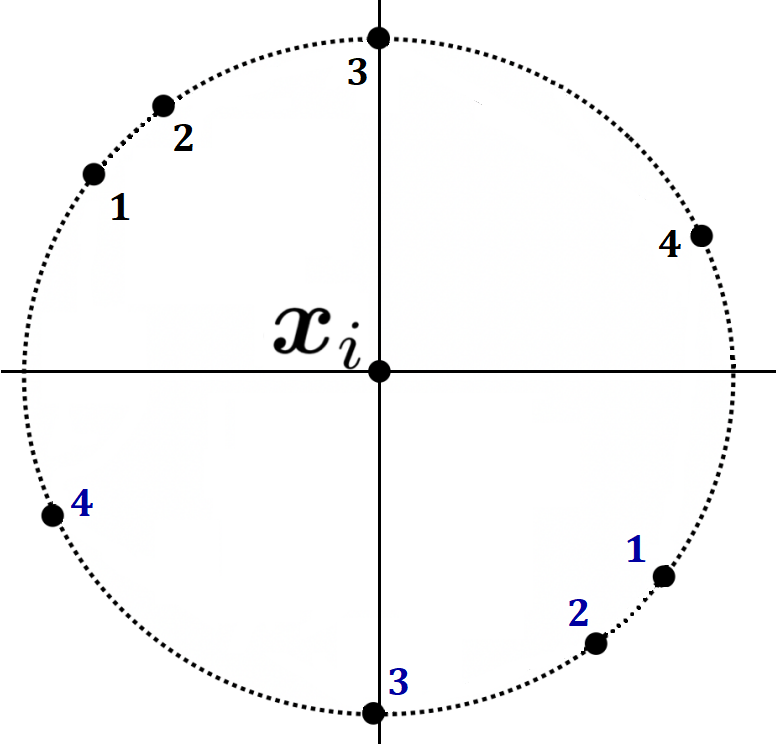
For a particular xᵢ, we define Sᵢ as the subset of S that includes only the points that represent labelings in which xᵢ is positively classified. Similarly, we derive the origin-symmetric Sᵢ’ ⊂ S’ from Sᵢ. In the example below, the points above the x-axis are those representing labelings in which xᵢ is positively classified, i.e., Sᵢ. Those below the x-axis comprise their origin-symmetric set Sᵢ’ (with the numbering matching between symmetric pairs of points). Note that the selection of points above the x-axis is completely arbitrary.
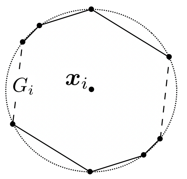
We proceed to construct a convex polygon Gᵢ, with its vertices being the points in Sᵢ ∪ Sᵢ’. The Gᵢ for each unlabeled data point will be key in designing an instance-wise cost function c with which we will always be able to achieve all possible labelings, thus showing that SVC(Hₗ, { 1 }, c) = ∞. Towards this end, the convexity of Gᵢ will prove critical, as will its origin symmetry (stemming from our choice of Sᵢ’ ).
Turning Polygons into Preferences: Constructing the Cost Function
For each of the n origin-initialized, unlabeled data points we started with, we now have a convex, origin-symmetric polygon that represents the labelings in which it is positively classified. Each Gᵢ can now be used to define the behavior of our instance-wise cost function c on its corresponding xᵢ. We will use Gᵢ to define a seminorm⁽³⁾:
∥ y ∥ɢᵢ = inf { ε ∈ ℝ⁺ : y ∈ εGᵢ }
This definition implies that the distance between xᵢ and some point z is less than 1 if and only if z lies within Gᵢ. I.e.:
∥ z – xᵢ ∥ɢᵢ < 1 ⇔ z ∈ Gᵢ
For the rest of the proof, it is sufficient that we understand this connection between ∥ ⋅ ∥ɢᵢ and a point being inside Gᵢ. (See Footnote (3) for a discussion of why ∥ ⋅ ∥ɢᵢ qualifies as a seminorm and for more details about its geometric interpretation.)
We thus define the instance-wise cost function c:
c(z; xᵢ) = ℓᵢ(z – xᵢ)
Where:
ℓᵢ(z – xᵢ) = ∥ z – xᵢ ∥ɢᵢ
That is, for each unlabeled data point xᵢ, c behaves as ∥ ⋅ ∥ɢᵢ would. Note that this behavior is different for each data point. This is because we constructed a unique Gᵢ for every xᵢ, and each ∥ ⋅ ∥ɢᵢ is derived from its corresponding polygon Gᵢ.
Data Point Best Response as a Result of the Cost Function
With the instance-wise cost function c in place, we may turn our attention to how our data points interact with linear classifiers. Recall that we have constrained our consideration to the homogeneous preference class, meaning that r = 1 for all of our points. I.e., xᵢ stands to gain a reward of magnitude 1 for being positively classified. Given a linear classifier, each data point will thus be willing to incur any cost less than 1 to manipulate its feature vector to ensure it falls on the positive side of the decision boundary. This will guarantee it receives positive utility as a result of the manipulation.
c is designed so that a data point with feature vector xᵢ has to pay ∥ z – xᵢ ∥ɢᵢ to change its feature vector to z. As we saw, as long as z lies inside Gᵢ, this cost will be less than 1.
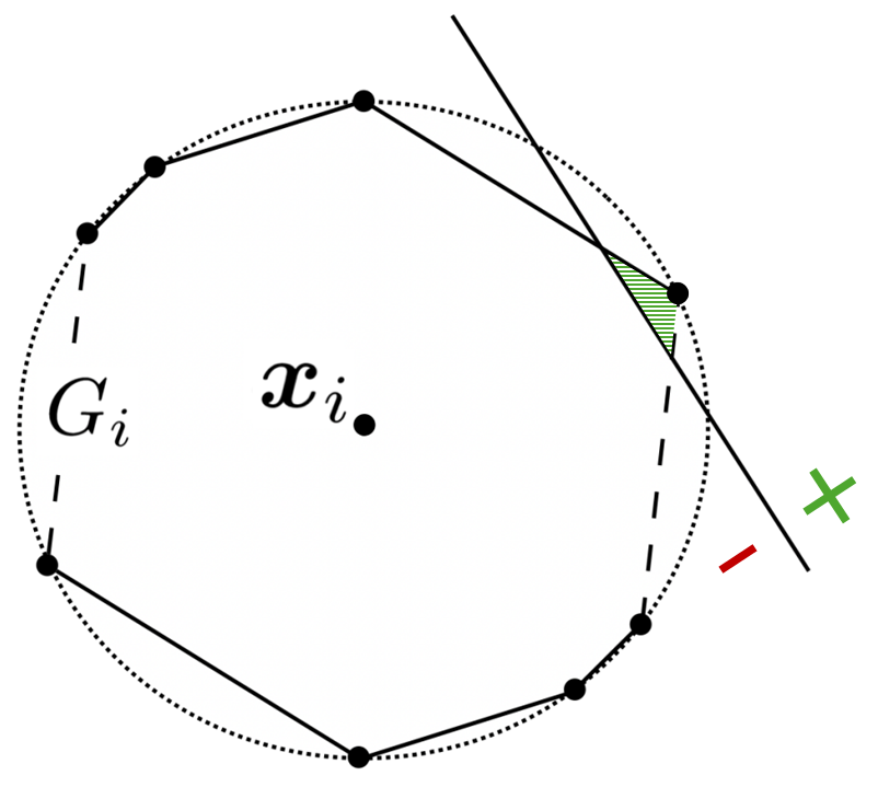
Suppose we have a decision boundary that crosses Gᵢ (intersects it at two points) with xᵢ falling on its negative half-plane. As illustrated in Figure 3 below, this creates a sub-polygon such that for any z within it:
- The cost to move to z is less than 1: c(z; xᵢ) = ∥ z — xᵢ ∥ɢᵢ < 1
- The realized reward for moving is precisely 1: 𝕀(h(z) = 1) ⋅ r = 1
Whereby the utility for data point i, 𝕀(h(z) = 1) ⋅ r – c(z; xᵢ), is positive, in turn making any such z a better response than non-manipulation. In other words, the data point will always want to manipulate its feature vector into one that lies in this sub-polygon.
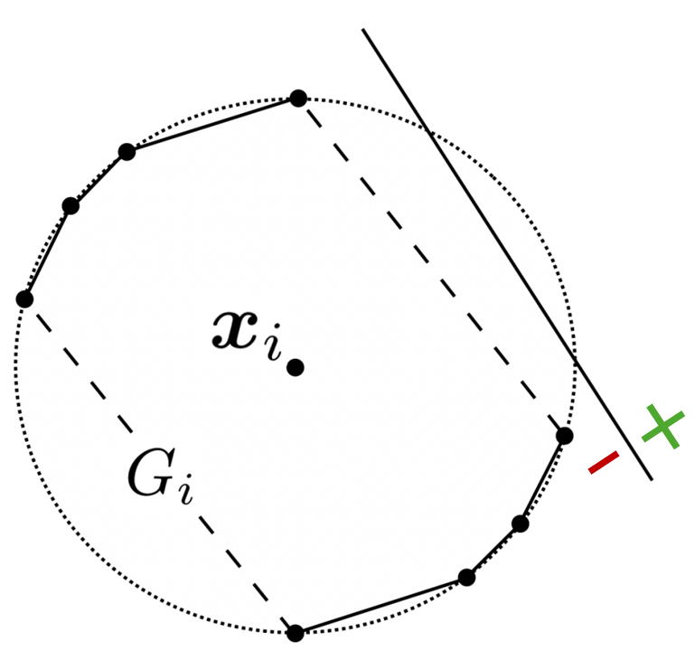
Conversely, given a decision boundary that does not cross Gᵢ, no such sub-polygon exists. The cost of manipulating xᵢ to cross the boundary will always be greater than 1, and thus not worth the reward. The data point best response will be the original feature vector, meaning it’s best to stay put.
Isolating Representative Points Using Linear Classifiers
We now understand the strategic implications of whether or not a certain decision boundary crosses Gᵢ. Calling to mind the role of our points on the unit circle as representatives of possible labelings, we can demonstrate the connection between labelings where a data point is positively classified and linear classifiers.
Let 𝓛 be an arbitrary labeling of our n data points, and let sₗ ∈ S be its unique representative point on the unit circle. Let xᵢ be one of our unlabeled data points. We will explore the behavior of the data point with respect to a particular linear classifier, denoted hₗ. We require that the decision boundary induced by hₗ do the following:
- Cross the unit circle.
- Strictly separate sₗ from all other points in S ∪ S’.
- Positively classify sₗ.
The structure of S ∪ S’ guarantees that such an hₗ exists.⁽⁴⁾
With hₗ at our disposal, we may explore how our cost function c interacts with hₗ for xᵢ depending on whether or not xᵢ should be positively classified under 𝓛. In fact, we will prove that a data point is positively classified by hₗ if and only if it is positively labeled under 𝓛.
Let us first consider the case in which we want xᵢ to be positively labeled (see Figure 5). Recall that we defined Sᵢ as “the subset of S that includes only the points that represent labelings in which xᵢ is positively classified.” We know, then, that sₗ ∈ Sᵢ. In particular, sₗ must be one of the vertices of Gᵢ. The fact that hₗ strictly separates sₗ from all other points in S ∪ S’ means that it is strictly separated from the other vertices of Gᵢ. Hence, hₗ must cross Gᵢ, incentivizing the data point to manipulate its feature vector.
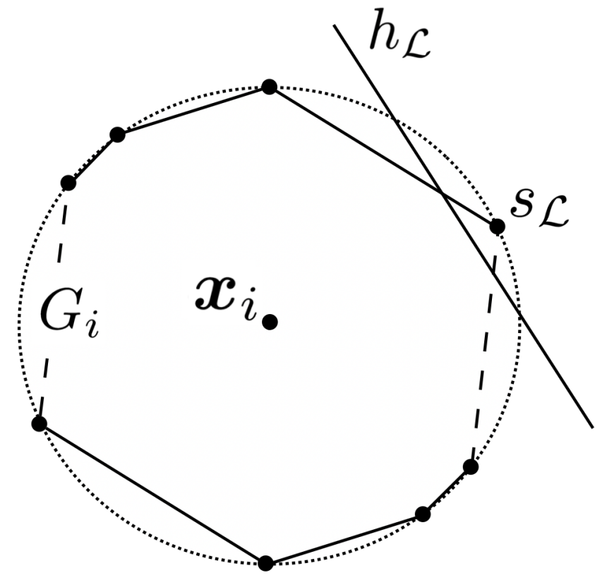
We proceed to examine the case in which we want xᵢ to be negatively labeled under 𝓛 (see Figure 6). As a result of how we constructed Sᵢ, sₗ ∉ Sᵢ. Additionally, having required that the origin-symmetric S’ be disjoint from S, we know that sₗ ∉ Sᵢ’. It follows that sₗ is not a vertex of Gᵢ. Once again, hₗ strictly separates sₗ from all other points in S ∪ S’, including all the vertices of Gᵢ. Because Gᵢ is convex, we conclude that any point in Gᵢ is on the opposite side of hₗ as sₗ. In other words, hₗ does not cross Gᵢ. Consequently, the data point will choose to stay put rather than “overpaying” to manipulate its feature vector to cross hₗ.
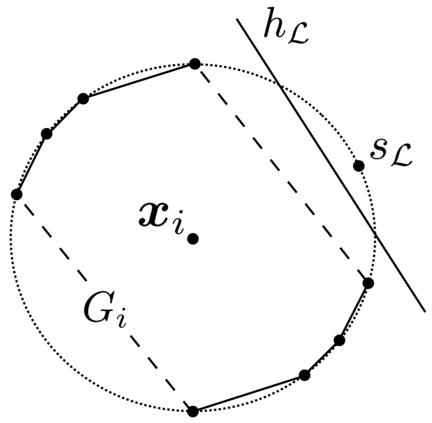
In summary, our unlabeled data point xᵢ will engage in manipulation to cross hₗ if and only if 𝓛 dictates that the data point should be positively classified. In our strategic classification setting, this means that hₗ positively classifies a data point if and only if that data point should be positively labeled according to 𝓛.
Putting It All Together: Inducing an Arbitrary Labeling
Using what we have seen so far, we are able to demonstrate that we can achieve any labeling of our n data points we want. Overlaying all of our data points and their respective polygons (see Figure 7), we can see that given a labeling 𝓛, we are able to achieve it with the help of a corresponding linear classifier hₗ.
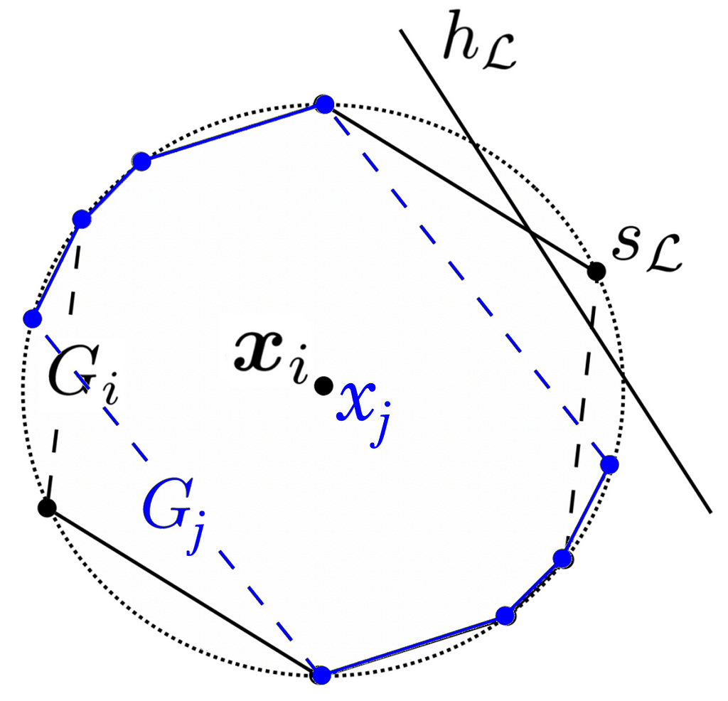
Any data point xᵢ that 𝓛 rules should be positively classified will manipulate its feature vector and move to the positive side of the decision boundary created by hₗ (like the case in Figure 5). At the same time, any data point xⱼ that should be negatively classified will not be sufficiently incentivized to manipulate its feature vector, causing it to stay on the negative side of the decision boundary. Across all n data points, those that will be positively classified will be exactly the ones that 𝓛 dictates should be positively classified. In other words, we can induce any labeling we wish.
We therefore have a sample of n unlabeled, potentially-manipulated data points that is strategically shattered by Hₗ, the hypothesis class of all linear classifiers in ℝ². Based on how we defined strategic shattering coefficients, we find that σₙ(Hₗ, { 1 }, c) = 2ⁿ. It follows that SVC(Hₗ, { 1 }, c) = ∞.
Conclusion
First, we posed linear classification as a problem that is canonically PAC learnable, but not generally strategic PAC learnable. Second, we simplified our strategic classification problem by limiting our consideration to the homogeneous preference class on the Cartesian plane. Given n origin-initialized data points, we mapped each of their 2ⁿ possible labelings to a unique representative point on the unit circle. We then created a polygon for each data point using the representative points corresponding to the labelings under which it should be positively classified.
Based on those polygons, we constructed an instance-wise cost function, c, for which the cost of feature manipulation is less than 1 only within each polygon. Next, we showed that for any labeling 𝓛, we could find a linear classifier that isolates its respective representative point. Such a classifier, paired with c, ensured that only the data points that are supposed to be positively classified according to 𝓛 are incentivized to manipulate their feature vectors to cross the decision boundary and end up with a positive label. Finally, we explained why that means that the SVC of the problem is infinite.
Acknowledgments
Writing this series of articles has been a wonderful journey, and I’m truly grateful to everyone who took the time to read them, especially those who reached out with feedback. This series wouldn’t have been possible without the authors of PAC-Learning for Strategic Classification: Ravi Sundaram, Anil Vullikanti, Haifeng Xu, and Fan Yao. They set the stage beautifully for a deep dive into this fascinating meeting point between machine learning and game theory. Thank you to the TDS Editors, particularly Ben Huberman and Ludovic Benistant, for their support and for giving me such a fantastic platform to share my writing. Lastly, a huge thank you to Prof. Inbal Talgam-Cohen for sowing the seeds that grew into this series in the seminar she taught last winter.
If you enjoyed these articles, please consider following me on Medium and LinkedIn to keep up with future articles and projects.
Footnotes
(1) See a proof of this result, as well as a great interactive explanation of linear classification, here. What we refer to as a “linear classifier” throughout this article is technically an affine classifier.
(2) Indeed, the paper shows that restricting our consideration to instance-invariant cost functions yields a problem that is PAC learnable, just like the in the canonical setting. For a refresher on the difference between instance-invariant and instance-wise cost functions, see the first article in this series.
(3) ∥ ⋅ ∥ɢᵢ as we defined it is the Minkowski functional of Gᵢ. In this context, we view Gᵢ as the set of points enclosed in the polygon we constructed. The Minkowski functional generalizes the notion of a seminorm. Recall that in the first article in this series, we assumed our cost function is induced by seminorms. We would be remiss not to reconcile this assumption with the construction of ∥ ⋅ ∥ɢᵢ.
Fortunately, it can be proven that the Minkowski functional of a set A is a seminorm under certain conditions [2]:
- A is a subset of a vector space over ℝ.
- A is convex.
- A is symmetric.
- A is an absorbing set.
Even more fortunately (or rather, by meticulous design), Gᵢ fulfills all of these conditions:
- Gᵢ is a subset of ℝ², which is a vector space over ℝ.
- Gᵢ is a convex set since it is bounded by a convex polygon.
- Gᵢ is origin-symmetric. (This is why we needed the Sᵢ’ in the first place!)
- Gᵢ is a convex subset of the topological vector space ℝ² equipped with the standard topology induced by the Euclidean norm. Gᵢ also contains the origin in its interior. Therefore, Gᵢ is an absorbing set [3].
∥ ⋅ ∥ɢᵢ is therefore a seminorm for all i, enabling us to continue the proof without violating our assumptions.
(4) Let P be the convex hull of (S ∪ S’) sₗ. Note that S ∪ S’ is finite. It can be proven that the convex hull of a finite set in ℝ² is compact [4]. As a singleton, { sₗ } is closed. Clearly, (S ∪ S’) sₗ and sₗ are disjoint. It follows from the hyperplane separation theorem that there exists a hyperplane that strictly separates the two.
Let us also show that the linear decision boundary induced by the aforementioned hyperplane must intersect the unit circle at two points. Recall that a line may intersect a circle at exactly zero, one, or two points.
- Suppose for the sake of contradiction that the decision boundary and the unit circle are disjoint. Then all points in the unit circle must lie on the same side of the decision boundary, contradicting the assumption that hₗ separates (S ∪ S’) sₗ from sₗ.
- Due to the fact that the separation is strict, sₗ may not lie on the decision boundary, whereby the latter cannot be tangent to the unit circle.
- The only remaining possibility is that the decision boundary crosses the unit circle.
As for ensuring hₗ positively classifies sₗ, it is completely up to us which side of the boundary we wish to classify positively.
References
[1] R. Sundaram, A. Vullikanti, H. Xu, F. Yao. PAC-Learning for Strategic Classification (2021), International Conference on Machine Learning.
[2] ProofWiki contributors. Minkowski functional of symmetric convex absorbing set in real vector space is seminorm.
[3] ProofWiki contributors. Convex subset of topological vector space containing zero vector in interior is absorbing set.
[4] Math Stack Exchange contributors. Is convex hull of a finite set of points in R² closed?
Statistical Learnability of Strategic Linear Classifiers: A Proof Walkthrough was originally published in Towards Data Science on Medium, where people are continuing the conversation by highlighting and responding to this story.
With the help of an intricate geometric construction, we can prove that instance-wise cost functions quickly drive SVC to infinity.In the previous article in this series, we examined the concept of strategic VC dimension (SVC) and its connection to the Fundamental Theorem of Strategic Learning. We will make use of both of those in this article, alongside the ideas of achievable labelings and strategic shattering coefficients that we explored in the lead-up to them.Quantifying the Complexity and Learnability of Strategic Classification ProblemsIf you haven’t read the first article in this series yet, I encourage you to start from there before moving on to the aforementioned article on SVC:Extending PAC Learning to a Strategic Classification SettingWith the context from the other articles in this series in place, a basic grasp of set theory and geometry will be all you’ll need to understand the theorem and its proof.How an Instance-Wise Cost Function Affects SVC: Stating the TheoremAs we saw, SVC can be used as a tool to estimate the expressive power of a hypothesis class within a strategic classification context. Having carefully defined SVC as a generalization of the canonical VC dimension, we understand that the two have much in common. When, though, does SVC diverge from its canonical counterpart? Can we come up with a scenario in which the strategic aspect of a classification problem significantly increases its complexity? It turns out we can, with relative ease: linear classification.Linear classification involves determining whether a data point should be positively or negatively classified based on a linear function applied to its features. Geometrically, we can imagine a linear classifier inducing a linear decision boundary in d-dimensional real space (ℝᵈ ). Anything on one side of the boundary is positively classified, and anything on the other side is negatively classified. In one-dimensional space, the decision boundary is a threshold (as we saw in the previous article). In two-dimensional space, it’s a line dividing the plane. In general, it’s a hyperplane.In canonical binary classification, the VC dimension of the hypothesis class comprising all linear classifiers in ℝᵈ is d + 1, which is finite. For example, for d = 2 (linear classifiers in ℝ²), the VC dimension is 3. The Fundamental Theorem of Statistical Learning dictates that canonical linear classification is therefore PAC learnable.⁽¹⁾Intuitively, we might expect the same conclusion to hold for the strategic analog of the problem. After all, linear classifiers are some of the simplest classifiers there are, and reasoning about them can be rather natural.⁽²⁾However, that simplicity goes out the window as soon as we throw instance-wise cost functions into the mix. As we will prove:Given a strategic linear classification problem Sᴛʀᴀᴄ⟨H, R, c⟩, there exists an instance-wise cost function c(z; x) = ℓₓ(z – x) such that SVC(H, R, c) = ∞.In other words, using the Fundamental Theorem of Strategic Learning, we find that linear classification in a strategic setting equipped with an instance-wise cost function is not generally PAC learnable. Interestingly, it will not be PAC learnable even if we strip away as much complexity as we can. In this case, we will do so by focusing on strategic linear classification on the Cartesian plane ( X ⊆ ℝ²) with the homogeneous preference class (R = { 1 }).The more general conclusion will follow from the counterexample we will show under those simplifying conditions. If strategic linear classification is not PAC learnable in ℝ², there is no way it could be PAC learnable in any higher dimension. Likewise, every other preference class we laid out in our setup is a strict generalization of the homogeneous preference class. If we could prove PAC learnability for any of those preference classes, we would also be able to do so for the simpler case where R = { 1 }.From Labelings to Points on the Unit Circle: Proof SetupBased on the assumptions above, we begin by turning our attention to the special case Sᴛʀᴀᴄ⟨Hₗ, { 1 }, c⟩, with Hₗ being the hypothesis class comprising all linear classifiers in ℝ². We then initialize n two-dimensional feature vectors at the origin: ∀ i ≤ n . xᵢ = (0, 0). Since we’re using the homogeneous preference class, we have that ∀ i ≤ n . rᵢ = 1. The only difference between the data points will be in how our cost function behaves on each of them. This is where the crux of the proof lies, as we will soon see.Before we discuss the cost function at length, though, we need to geometrize the possible labelings of our unlabeled data points. As we saw last time, a set of n unlabeled data points must have exactly 2ⁿ possible labelings. Representing a set of labelings (n-tuples) geometrically in ℝ² is relatively straightforward: we simply select an arbitrary point for each possible labeling. In particular, we will choose 2ⁿ such representative points on the unit circle, each assigned to a possible labeling. While the particular coordinates of the representative points themselves are unimportant, we do require that each such point be unique. We also require that no two points be origin-symmetric with respect to one another.We will denote this set of representative points by S. Having selected our representative points, we use them to define the origin-symmetric set S’, i.e., S’ = { (-x, -y) : (x, y) ∈ S }. Note that S and S’ are disjoint (S ∩ S’ = ∅) as a consequence of how we selected the points in S.For a particular xᵢ, we define Sᵢ as the subset of S that includes only the points that represent labelings in which xᵢ is positively classified. Similarly, we derive the origin-symmetric Sᵢ’ ⊂ S’ from Sᵢ. In the example below, the points above the x-axis are those representing labelings in which xᵢ is positively classified, i.e., Sᵢ. Those below the x-axis comprise their origin-symmetric set Sᵢ’ (with the numbering matching between symmetric pairs of points). Note that the selection of points above the x-axis is completely arbitrary.Figure 1: An example of labeling geometrization for an arbitrary xᵢ. Recall that we started by initializing all unlabeled data points as (0, 0). Points in Sᵢ are numbered in black. Their origin-symmetric counterparts in Sᵢ’ are numbered in blue. Image by the author, based on image by R. Sundaram, A. Vullikanti, H. Xu, F. Yao from PAC-Learning for Strategic Classification (use under CC-BY 4.0 license).We proceed to construct a convex polygon Gᵢ, with its vertices being the points in Sᵢ ∪ Sᵢ’. The Gᵢ for each unlabeled data point will be key in designing an instance-wise cost function c with which we will always be able to achieve all possible labelings, thus showing that SVC(Hₗ, { 1 }, c) = ∞. Towards this end, the convexity of Gᵢ will prove critical, as will its origin symmetry (stemming from our choice of Sᵢ’ ).Figure 2: The convex, origin-symmetric polygon Gᵢ derived from Sᵢ and Sᵢ’ as shown in Figure 1. Image by the author, based on image by R. Sundaram, A. Vullikanti, H. Xu, F. Yao from PAC-Learning for Strategic Classification (use under CC-BY 4.0 license).Turning Polygons into Preferences: Constructing the Cost FunctionFor each of the n origin-initialized, unlabeled data points we started with, we now have a convex, origin-symmetric polygon that represents the labelings in which it is positively classified. Each Gᵢ can now be used to define the behavior of our instance-wise cost function c on its corresponding xᵢ. We will use Gᵢ to define a seminorm⁽³⁾:∥ y ∥ɢᵢ = inf { ε ∈ ℝ⁺ : y ∈ εGᵢ }This definition implies that the distance between xᵢ and some point z is less than 1 if and only if z lies within Gᵢ. I.e.:∥ z – xᵢ ∥ɢᵢ < 1 ⇔ z ∈ GᵢFor the rest of the proof, it is sufficient that we understand this connection between ∥ ⋅ ∥ɢᵢ and a point being inside Gᵢ. (See Footnote (3) for a discussion of why ∥ ⋅ ∥ɢᵢ qualifies as a seminorm and for more details about its geometric interpretation.)We thus define the instance-wise cost function c:c(z; xᵢ) = ℓᵢ(z – xᵢ)Where:ℓᵢ(z – xᵢ) = ∥ z – xᵢ ∥ɢᵢThat is, for each unlabeled data point xᵢ, c behaves as ∥ ⋅ ∥ɢᵢ would. Note that this behavior is different for each data point. This is because we constructed a unique Gᵢ for every xᵢ, and each ∥ ⋅ ∥ɢᵢ is derived from its corresponding polygon Gᵢ.Data Point Best Response as a Result of the Cost FunctionWith the instance-wise cost function c in place, we may turn our attention to how our data points interact with linear classifiers. Recall that we have constrained our consideration to the homogeneous preference class, meaning that r = 1 for all of our points. I.e., xᵢ stands to gain a reward of magnitude 1 for being positively classified. Given a linear classifier, each data point will thus be willing to incur any cost less than 1 to manipulate its feature vector to ensure it falls on the positive side of the decision boundary. This will guarantee it receives positive utility as a result of the manipulation.c is designed so that a data point with feature vector xᵢ has to pay ∥ z – xᵢ ∥ɢᵢ to change its feature vector to z. As we saw, as long as z lies inside Gᵢ, this cost will be less than 1.Suppose we have a decision boundary that crosses Gᵢ (intersects it at two points) with xᵢ falling on its negative half-plane. As illustrated in Figure 3 below, this creates a sub-polygon such that for any z within it:The cost to move to z is less than 1: c(z; xᵢ) = ∥ z — xᵢ ∥ɢᵢ < 1The realized reward for moving is precisely 1: 𝕀(h(z) = 1) ⋅ r = 1Whereby the utility for data point i, 𝕀(h(z) = 1) ⋅ r – c(z; xᵢ), is positive, in turn making any such z a better response than non-manipulation. In other words, the data point will always want to manipulate its feature vector into one that lies in this sub-polygon.Figure 3: An example of a linear classifier with a decision boundary that properly intersects Gᵢ, with xᵢ falling on its negative half-plane. The resulting “Goldilocks zone” between the decision boundary and the perimeter of Gᵢ is shaded in green. Changing xᵢ to any z lying in this area confers positive utility. This is because the reward gained is 1 and the cost incurred is less than 1. Image by the author, based on image by R. Sundaram, A. Vullikanti, H. Xu, F. Yao from PAC-Learning for Strategic Classification (use under CC-BY 4.0 license).Conversely, given a decision boundary that does not cross Gᵢ, no such sub-polygon exists. The cost of manipulating xᵢ to cross the boundary will always be greater than 1, and thus not worth the reward. The data point best response will be the original feature vector, meaning it’s best to stay put.Figure 4: An example of a polygon Gᵢ and a linear classifier with a decision boundary that does not cross it. Note how there are no points that are both on the positive side of the decision boundary and inside Gᵢ. Equivalently, there are no vectors into which the data point could manipulate its feature vector for positive utility. Image by the author, based on image by R. Sundaram, A. Vullikanti, H. Xu, F. Yao from PAC-Learning for Strategic Classification (use under CC-BY 4.0 license).Isolating Representative Points Using Linear ClassifiersWe now understand the strategic implications of whether or not a certain decision boundary crosses Gᵢ. Calling to mind the role of our points on the unit circle as representatives of possible labelings, we can demonstrate the connection between labelings where a data point is positively classified and linear classifiers.Let 𝓛 be an arbitrary labeling of our n data points, and let sₗ ∈ S be its unique representative point on the unit circle. Let xᵢ be one of our unlabeled data points. We will explore the behavior of the data point with respect to a particular linear classifier, denoted hₗ. We require that the decision boundary induced by hₗ do the following:Cross the unit circle.Strictly separate sₗ from all other points in S ∪ S’.Positively classify sₗ.The structure of S ∪ S’ guarantees that such an hₗ exists.⁽⁴⁾With hₗ at our disposal, we may explore how our cost function c interacts with hₗ for xᵢ depending on whether or not xᵢ should be positively classified under 𝓛. In fact, we will prove that a data point is positively classified by hₗ if and only if it is positively labeled under 𝓛.Let us first consider the case in which we want xᵢ to be positively labeled (see Figure 5). Recall that we defined Sᵢ as “the subset of S that includes only the points that represent labelings in which xᵢ is positively classified.” We know, then, that sₗ ∈ Sᵢ. In particular, sₗ must be one of the vertices of Gᵢ. The fact that hₗ strictly separates sₗ from all other points in S ∪ S’ means that it is strictly separated from the other vertices of Gᵢ. Hence, hₗ must cross Gᵢ, incentivizing the data point to manipulate its feature vector.Figure 5: If xᵢ should be positively labeled under 𝓛, hₗ crosses Gᵢ. This incentivizes the data point to manipulate its feature vector (see Figure 3). Image by R. Sundaram, A. Vullikanti, H. Xu, F. Yao from PAC-Learning for Strategic Classification (use under CC-BY 4.0 license).We proceed to examine the case in which we want xᵢ to be negatively labeled under 𝓛 (see Figure 6). As a result of how we constructed Sᵢ, sₗ ∉ Sᵢ. Additionally, having required that the origin-symmetric S’ be disjoint from S, we know that sₗ ∉ Sᵢ’. It follows that sₗ is not a vertex of Gᵢ. Once again, hₗ strictly separates sₗ from all other points in S ∪ S’, including all the vertices of Gᵢ. Because Gᵢ is convex, we conclude that any point in Gᵢ is on the opposite side of hₗ as sₗ. In other words, hₗ does not cross Gᵢ. Consequently, the data point will choose to stay put rather than “overpaying” to manipulate its feature vector to cross hₗ.Figure 6: If xᵢ should be positively labeled under 𝓛, hₗ does not cross Gᵢ. This incentivizes the data point not to manipulate its feature vector (see Figure 4). Image by R. Sundaram, A. Vullikanti, H. Xu, F. Yao from PAC-Learning for Strategic Classification (use under CC-BY 4.0 license).In summary, our unlabeled data point xᵢ will engage in manipulation to cross hₗ if and only if 𝓛 dictates that the data point should be positively classified. In our strategic classification setting, this means that hₗ positively classifies a data point if and only if that data point should be positively labeled according to 𝓛.Putting It All Together: Inducing an Arbitrary LabelingUsing what we have seen so far, we are able to demonstrate that we can achieve any labeling of our n data points we want. Overlaying all of our data points and their respective polygons (see Figure 7), we can see that given a labeling 𝓛, we are able to achieve it with the help of a corresponding linear classifier hₗ.Figure 7: Simplified visualization of overlaid data points with their corresponding cost function polygons. sₗ represents a labeling 𝓛 in which data point i should be positively classified and data point j should be negatively classified. The unmanipulated feature vectors of the two overlap at (0, 0). However, data point i will be positively classified by hₗ because it will move to the positive side of the decision boundary induced by hₗ (since the boundary crosses Gᵢ). Data point j will stay on the negative side because the boundary does not cross Gⱼ. Image by the author, based on images by R. Sundaram, A. Vullikanti, H. Xu, F. Yao from PAC-Learning for Strategic Classification (use under CC-BY 4.0 license).Any data point xᵢ that 𝓛 rules should be positively classified will manipulate its feature vector and move to the positive side of the decision boundary created by hₗ (like the case in Figure 5). At the same time, any data point xⱼ that should be negatively classified will not be sufficiently incentivized to manipulate its feature vector, causing it to stay on the negative side of the decision boundary. Across all n data points, those that will be positively classified will be exactly the ones that 𝓛 dictates should be positively classified. In other words, we can induce any labeling we wish.We therefore have a sample of n unlabeled, potentially-manipulated data points that is strategically shattered by Hₗ, the hypothesis class of all linear classifiers in ℝ². Based on how we defined strategic shattering coefficients, we find that σₙ(Hₗ, { 1 }, c) = 2ⁿ. It follows that SVC(Hₗ, { 1 }, c) = ∞.ConclusionFirst, we posed linear classification as a problem that is canonically PAC learnable, but not generally strategic PAC learnable. Second, we simplified our strategic classification problem by limiting our consideration to the homogeneous preference class on the Cartesian plane. Given n origin-initialized data points, we mapped each of their 2ⁿ possible labelings to a unique representative point on the unit circle. We then created a polygon for each data point using the representative points corresponding to the labelings under which it should be positively classified.Based on those polygons, we constructed an instance-wise cost function, c, for which the cost of feature manipulation is less than 1 only within each polygon. Next, we showed that for any labeling 𝓛, we could find a linear classifier that isolates its respective representative point. Such a classifier, paired with c, ensured that only the data points that are supposed to be positively classified according to 𝓛 are incentivized to manipulate their feature vectors to cross the decision boundary and end up with a positive label. Finally, we explained why that means that the SVC of the problem is infinite.AcknowledgmentsWriting this series of articles has been a wonderful journey, and I’m truly grateful to everyone who took the time to read them, especially those who reached out with feedback. This series wouldn’t have been possible without the authors of PAC-Learning for Strategic Classification: Ravi Sundaram, Anil Vullikanti, Haifeng Xu, and Fan Yao. They set the stage beautifully for a deep dive into this fascinating meeting point between machine learning and game theory. Thank you to the TDS Editors, particularly Ben Huberman and Ludovic Benistant, for their support and for giving me such a fantastic platform to share my writing. Lastly, a huge thank you to Prof. Inbal Talgam-Cohen for sowing the seeds that grew into this series in the seminar she taught last winter.If you enjoyed these articles, please consider following me on Medium and LinkedIn to keep up with future articles and projects.Footnotes(1) See a proof of this result, as well as a great interactive explanation of linear classification, here. What we refer to as a “linear classifier” throughout this article is technically an affine classifier.(2) Indeed, the paper shows that restricting our consideration to instance-invariant cost functions yields a problem that is PAC learnable, just like the in the canonical setting. For a refresher on the difference between instance-invariant and instance-wise cost functions, see the first article in this series.(3) ∥ ⋅ ∥ɢᵢ as we defined it is the Minkowski functional of Gᵢ. In this context, we view Gᵢ as the set of points enclosed in the polygon we constructed. The Minkowski functional generalizes the notion of a seminorm. Recall that in the first article in this series, we assumed our cost function is induced by seminorms. We would be remiss not to reconcile this assumption with the construction of ∥ ⋅ ∥ɢᵢ.Fortunately, it can be proven that the Minkowski functional of a set A is a seminorm under certain conditions [2]:A is a subset of a vector space over ℝ.A is convex.A is symmetric.A is an absorbing set.Even more fortunately (or rather, by meticulous design), Gᵢ fulfills all of these conditions:Gᵢ is a subset of ℝ², which is a vector space over ℝ.Gᵢ is a convex set since it is bounded by a convex polygon.Gᵢ is origin-symmetric. (This is why we needed the Sᵢ’ in the first place!)Gᵢ is a convex subset of the topological vector space ℝ² equipped with the standard topology induced by the Euclidean norm. Gᵢ also contains the origin in its interior. Therefore, Gᵢ is an absorbing set [3].∥ ⋅ ∥ɢᵢ is therefore a seminorm for all i, enabling us to continue the proof without violating our assumptions.(4) Let P be the convex hull of (S ∪ S’) sₗ. Note that S ∪ S’ is finite. It can be proven that the convex hull of a finite set in ℝ² is compact [4]. As a singleton, { sₗ } is closed. Clearly, (S ∪ S’) sₗ and sₗ are disjoint. It follows from the hyperplane separation theorem that there exists a hyperplane that strictly separates the two.Let us also show that the linear decision boundary induced by the aforementioned hyperplane must intersect the unit circle at two points. Recall that a line may intersect a circle at exactly zero, one, or two points.Suppose for the sake of contradiction that the decision boundary and the unit circle are disjoint. Then all points in the unit circle must lie on the same side of the decision boundary, contradicting the assumption that hₗ separates (S ∪ S’) sₗ from sₗ.Due to the fact that the separation is strict, sₗ may not lie on the decision boundary, whereby the latter cannot be tangent to the unit circle.The only remaining possibility is that the decision boundary crosses the unit circle.As for ensuring hₗ positively classifies sₗ, it is completely up to us which side of the boundary we wish to classify positively.References[1] R. Sundaram, A. Vullikanti, H. Xu, F. Yao. PAC-Learning for Strategic Classification (2021), International Conference on Machine Learning.[2] ProofWiki contributors. Minkowski functional of symmetric convex absorbing set in real vector space is seminorm.[3] ProofWiki contributors. Convex subset of topological vector space containing zero vector in interior is absorbing set.[4] Math Stack Exchange contributors. Is convex hull of a finite set of points in R² closed?Statistical Learnability of Strategic Linear Classifiers: A Proof Walkthrough was originally published in Towards Data Science on Medium, where people are continuing the conversation by highlighting and responding to this story. thoughts-and-theory, classification-algorithms, game-theory, machine-learning, vc-dimension Towards Data Science – MediumRead More

 Add to favorites


0 Comments