Using knowledge graphs and AI to retrieve, filter, and summarize medical journal articles
The accompanying code for the app and notebook are here.
Knowledge graphs (KGs) and Large Language Models (LLMs) are a match made in heaven. My previous posts discuss the complementarities of these two technologies in more detail but the short version is, “some of the main weaknesses of LLMs, that they are black-box models and struggle with factual knowledge, are some of KGs’ greatest strengths. KGs are, essentially, collections of facts, and they are fully interpretable.”
This article is all about building a simple Graph RAG app. What is RAG? RAG, or Retrieval-Augmented Generation, is about retrieving relevant information to augment a prompt that is sent to an LLM, which generates a response. Graph RAG is RAG that uses a knowledge graph as part of the retrieval portion. If you’ve never heard of Graph RAG, or want a refresher, I’d watch this video.
The basic idea is that, rather than sending your prompt directly to an LLM, which was not trained on your data, you can supplement your prompt with the relevant information needed for the LLM to answer your prompt accurately. The example I use often is copying a job description and my resume into ChatGPT to write a cover letter. The LLM is able to provide a much more relevant response to my prompt, ‘write me a cover letter,’ if I give it my resume and the description of the job I am applying for. Since knowledge graphs are built to store knowledge, they are a perfect way to store internal data and supplement LLM prompts with additional context, improving the accuracy and contextual understanding of the responses.
This technology has many, many, applications such customer service bots, drug discovery, automated regulatory report generation in life sciences, talent acquisition and management for HR, legal research and writing, and wealth advisor assistants. Because of the wide applicability and the potential to improve the performance of LLM tools, Graph RAG (that’s the term I’ll use here) has been blowing up in popularity. Here is a graph showing interest over time based on Google searches.
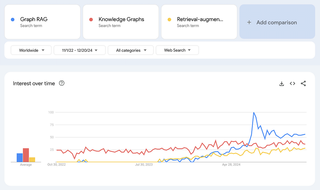
Graph RAG has experienced a surge in search interest, even surpassing terms like knowledge graphs and retrieval-augmented generation. Note that Google Trends measures relative search interest, not absolute number of searches. The spike in July 2024 for searches of Graph RAG coincides with the week Microsoft announced that their GraphRAG application would be available on GitHub.
The excitement around Graph RAG is broader than just Microsoft, however. Samsung acquired RDFox, a knowledge graph company, in July of 2024. The article announcing that acquisition did not mention Graph RAG explicitly, but in this article in Forbes published in November 2024, a Samsung spokesperson stated, “We plan to develop knowledge graph technology, one of the main technologies of personalized AI, and organically connect with generated AI to support user-specific services.”
In October 2024, Ontotext, a leading graph database company, and Semantic Web company, the maker of PoolParty, a knowledge graph curation platform, merged to form Graphwise. According to the press release, the merger aims to “democratize the evolution of Graph RAG as a category.”
While some of the buzz around Graph RAG may come from the broader excitement surrounding chatbots and generative AI, it reflects a genuine evolution in how knowledge graphs are being applied to solve complex, real-world problems. One example is that LinkedIn applied Graph RAG to improve their customer service technical support. Because the tool was able to retrieve the relevant data (like previously solved similar tickets or questions) to feed the LLM, the responses were more accurate and the mean resolution time dropped from 40 hours to 15 hours.
This post will go through the construction of a pretty simple, but I think illustrative, example of how Graph RAG can work in practice. The end result is an app that a non-technical user can interact with. Like my last post, I will use a dataset consisting of medical journal articles from PubMed. The idea is that this is an app that someone in the medical field could use to do literature review. The same principles can be applied to many use cases however, which is why Graph RAG is so exciting.
The structure of the app, along with this post is as follows:
Step zero is preparing the data. I will explain the details below but the overall goal is to vectorize the raw data and, separately, turn it into an RDF graph. As long as we keep URIs tied to the articles before we vectorize, we can navigate across a graph of articles and a vector space of articles. Then, we can:
- Search Articles: use the power of the vector database to do an initial search of relevant articles given a search term. I will use vector similarity to retrieve articles with the most similar vectors to that of the search term.
- Refine Terms: explore the Medical Subject Headings (MeSH) biomedical vocabulary to select terms to use to filter the articles from step 1. This controlled vocabulary contains medical terms, alternative names, narrower concepts, and many other properties and relationships.
- Filter & Summarize: use the MeSH terms to filter the articles to avoid ‘context poisoning’. Then send the remaining articles to an LLM along with an additional prompt like, “summarize in bullets.”
Some notes on this app and tutorial before we get started:
- This set-up uses knowledge graphs exclusively for metadata. This is only possible because each article in my dataset has already been tagged with terms that are part of a rich controlled vocabulary. I am using the graph for structure and semantics and the vector database for similarity-based retrieval, ensuring each technology is used for what it does best. Vector similarity can tell us “esophageal cancer” is semantically similar to “mouth cancer”, but knowledge graphs can tell us the details of the relationship between “esophageal cancer” and “mouth cancer.”
- The data I used for this app is a collection of medical journal articles from PubMed (more on the data below). I chose this dataset because it is structured (tabular) but also contains text in the form of abstracts for each article, and because it is already tagged with topical terms that are aligned with a well-established controlled vocabulary (MeSH). Because these are medical articles, I have called this app ‘Graph RAG for Medicine.’ But this same structure can be applied to any domain and is not specific to the medical field.
- What I hope this tutorial and app demonstrate is that you can improve the results of your RAG application in terms of accuracy and explainability by incorporating a knowledge graph into the retrieval step. I will show how KGs can improve the accuracy of RAG applications in two ways: by giving the user a way of filtering the context to ensure the LLM is only being fed the most relevant information; and by using domain specific controlled vocabularies with dense relationships that are maintained and curated by domain experts to do the filtering.
- What this tutorial and app don’t directly showcase are two other significant ways KGs can enhance RAG applications: governance, access control, and regulatory compliance; and efficiency and scalability. For governance, KGs can do more than filter content for relevancy to improve accuracy — they can enforce data governance policies. For instance, if a user lacks permission to access certain content, that content can be excluded from their RAG pipeline. On the efficiency and scalability side, KGs can help ensure RAG applications don’t die on the shelf. While it’s easy to create an impressive one-off RAG app (that’s literally the purpose of this tutorial), many companies struggle with a proliferation of disconnected POCs that lack a cohesive framework, structure, or platform. That means many of those apps are not going to survive long. A metadata layer powered by KGs can break down data silos, providing the foundation needed to build, scale, and maintain RAG applications effectively. Using a rich controlled vocabulary like MeSH for the metadata tags on these articles is a way of ensuring this Graph RAG app can be integrated with other systems and reducing the risk that it becomes a silo.
Step 0: Prepare the data
The code to prepare the data is in this notebook.
As mentioned, I’ve again decided to use this dataset of 50,000 research articles from the PubMed repository (License CC0: Public Domain). This dataset contains the title of the articles, their abstracts, as well as a field for metadata tags. These tags are from the Medical Subject Headings (MeSH) controlled vocabulary thesaurus. The PubMed articles are really just metadata on the articles — there are abstracts for each article but we don’t have the full text. The data is already in tabular format and tagged with MeSH terms.
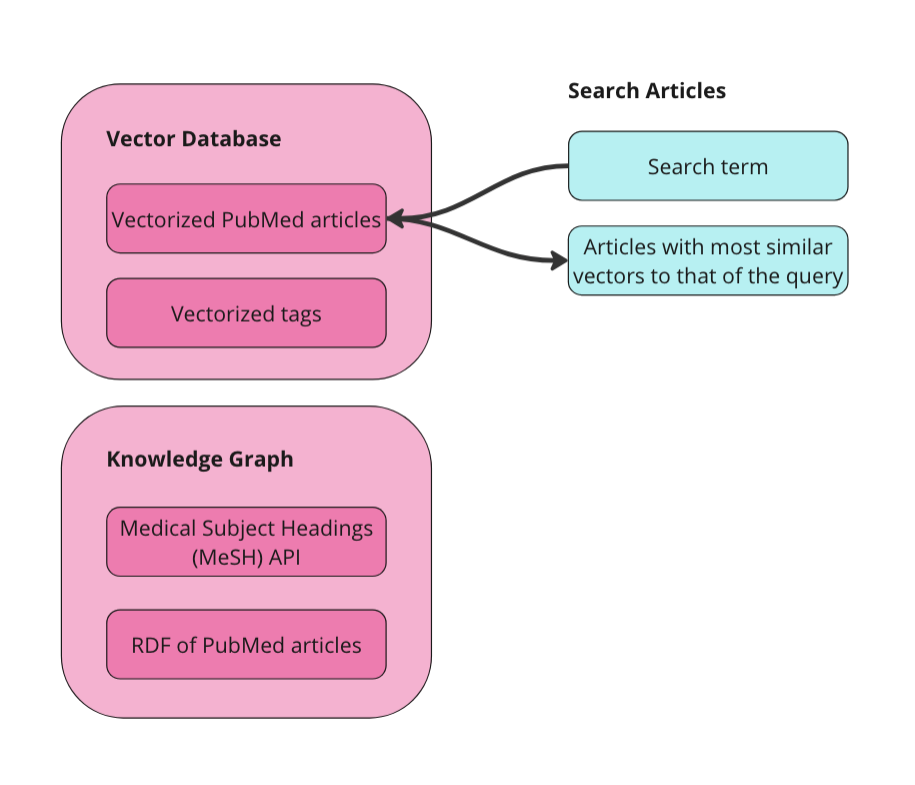
We can vectorize this tabular dataset directly. We could turn it into a graph (RDF) before we vectorize, but I didn’t do that for this app and I don’t know that it would help the final results for this kind of data. The most important thing about vectorizing the raw data is that we add Unique Resource Identifiers (URIs) to each article first. A URI is a unique ID for navigating RDF data and it is necessary for us to go back and forth between vectors and entities in our graph. Additionally, we will create a separate collection in our vector database for the MeSH terms. This will allow the user to search for relevant terms without having prior knowledge of this controlled vocabulary. Below is a diagram of what we are doing to prepare our data.
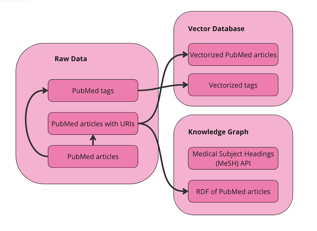
We have two collections in our vector database to query: articles and terms. We also have the data represented as a graph in RDF format. Since MeSH has an API, I am just going to query the API directly to get alternative names and narrower concepts for terms.
Vectorize data in Weaviate
First import the required packages and set up the Weaviate client:
import weaviate
from weaviate.util import generate_uuid5
from weaviate.classes.init import Auth
import os
import json
import pandas as pd

client = weaviate.connect_to_weaviate_cloud(
    cluster_url="XXX",  # Replace with your Weaviate Cloud URL
    auth_credentials=Auth.api_key("XXX"),  # Replace with your Weaviate Cloud key
    headers={'X-OpenAI-Api-key': "XXX"}  # Replace with your OpenAI API key
)
Read in the PubMed journal articles. I am using Databricks to run this notebook so you may need to change this, depending on where you run it. The goal here is just to get the data into a pandas DataFrame.
df = spark.sql("SELECT * FROM workspace.default.pub_med_multi_label_text_classification_dataset_processed").toPandas()
If you’re running this locally, just do:
df = pd.read_csv("PubMed Multi Label Text Classification Dataset Processed.csv")
Then clean the data up a bit:
import numpy as np
# Replace infinity values with NaN and then fill NaN values
df.replace([np.inf, -np.inf], np.nan, inplace=True)
df.fillna('', inplace=True)

# Convert columns to string type
df['Title'] = df['Title'].astype(str)
df['abstractText'] = df['abstractText'].astype(str)
df['meshMajor'] = df['meshMajor'].astype(str)
Now we need to create a URI for each article and add that in as a new column. This is important because the URI is the way we can connect the vector representation of an article with the knowledge graph representation of the article.
import urllib.parse
from rdflib import Graph, RDF, RDFS, Namespace, URIRef, Literal


# Function to create a valid URI
def create_valid_uri(base_uri, text):
    if pd.isna(text):
        return None
    # Encode text to be used in URI
    sanitized_text = urllib.parse.quote(text.strip().replace(' ', '_').replace('"', '').replace('<', '').replace('>', '').replace("'", "_"))
    return URIRef(f"{base_uri}/{sanitized_text}")


# Function to create a valid URI for Articles
def create_article_uri(title, base_namespace="http://example.org/article/"):
    """
    Creates a URI for an article by replacing non-word characters with underscores and URL-encoding.

    Args:
        title (str): The title of the article.
        base_namespace (str): The base namespace for the article URI.

    Returns:
        URIRef: The formatted article URI.
    """
    if pd.isna(title):
        return None
    # Replace non-word characters with underscores
    sanitized_title = re.sub(r'W+', '_', title.strip())
    # Condense multiple underscores into a single underscore
    sanitized_title = re.sub(r'_+', '_', sanitized_title)
    # URL-encode the term
    encoded_title = quote(sanitized_title)
    # Concatenate with base_namespace without adding underscores
    uri = f"{base_namespace}{encoded_title}"
    return URIRef(uri)

# Add a new column to the DataFrame for the article URIs
df['Article_URI'] = df['Title'].apply(lambda title: create_valid_uri("http://example.org/article", title))
We also want to create a DataFrame of all of the MeSH terms that are used to tag the articles. This will be helpful later when we want to search for similar MeSH terms.
# Function to clean and parse MeSH terms
def parse_mesh_terms(mesh_list):
    if pd.isna(mesh_list):
        return []
    return [
        term.strip().replace(' ', '_')
        for term in mesh_list.strip("[]'").split(',')
    ]

# Function to create a valid URI for MeSH terms
def create_valid_uri(base_uri, text):
    if pd.isna(text):
        return None
    sanitized_text = urllib.parse.quote(
        text.strip()
        .replace(' ', '_')
        .replace('"', '')
        .replace('<', '')
        .replace('>', '')
        .replace("'", "_")
    )
    return f"{base_uri}/{sanitized_text}"

# Extract and process all MeSH terms
all_mesh_terms = []
for mesh_list in df["meshMajor"]:
    all_mesh_terms.extend(parse_mesh_terms(mesh_list))

# Deduplicate terms
unique_mesh_terms = list(set(all_mesh_terms))

# Create a DataFrame of MeSH terms and their URIs
mesh_df = pd.DataFrame({
    "meshTerm": unique_mesh_terms,
    "URI": [create_valid_uri("http://example.org/mesh", term) for term in unique_mesh_terms]
})

# Display the DataFrame
print(mesh_df)
Vectorize the articles DataFrame:
from weaviate.classes.config import Configure


#define the collection
articles = client.collections.create(
    name = "Article",
    vectorizer_config=Configure.Vectorizer.text2vec_openai(),  # If set to "none" you must always provide vectors yourself. Could be any other "text2vec-*" also.
    generative_config=Configure.Generative.openai(),  # Ensure the `generative-openai` module is used for generative queries
)

#add ojects
articles = client.collections.get("Article")

with articles.batch.dynamic() as batch:
    for index, row in df.iterrows():
        batch.add_object({
            "title": row["Title"],
            "abstractText": row["abstractText"],
            "Article_URI": row["Article_URI"],
            "meshMajor": row["meshMajor"],
        })
Now vectorize the MeSH terms:
#define the collection
terms = client.collections.create(
    name = "term",
    vectorizer_config=Configure.Vectorizer.text2vec_openai(),  # If set to "none" you must always provide vectors yourself. Could be any other "text2vec-*" also.
    generative_config=Configure.Generative.openai(),  # Ensure the `generative-openai` module is used for generative queries
)

#add ojects
terms = client.collections.get("term")

with terms.batch.dynamic() as batch:
    for index, row in mesh_df.iterrows():
        batch.add_object({
            "meshTerm": row["meshTerm"],
            "URI": row["URI"],
        })
You can, at this point, run semantic search, similarity search, and RAG directly against the vectorized dataset. I won’t go through all of that here but you can look at the code in my accompanying notebook to do that.
Turn data into a knowledge graph
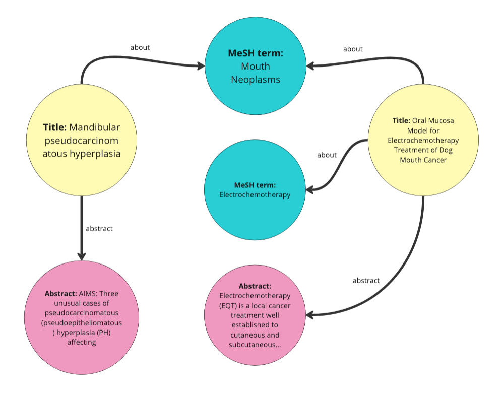
I am just using the same code we used in the last post to do this. We are basically turning every row in the data into an “Article” entity in our KG. Then we are giving each of these articles properties for title, abstract, and MeSH terms. We are also turning every MeSH term into an entity as well. This code also adds random dates to each article for a property called date published and a random number between 1 and 10 to a property called access. We won’t use those properties in this demo. Below is a visual representation of the graph we are creating from the data.
Here is how to iterate through the DataFrame and turn it into RDF data:
from rdflib import Graph, RDF, RDFS, Namespace, URIRef, Literal
from rdflib.namespace import SKOS, XSD
import pandas as pd
import urllib.parse
import random
from datetime import datetime, timedelta
import re
from urllib.parse import quote

# --- Initialization ---
g = Graph()

# Define namespaces
schema = Namespace('http://schema.org/')
ex = Namespace('http://example.org/')
prefixes = {
    'schema': schema,
    'ex': ex,
    'skos': SKOS,
    'xsd': XSD
}
for p, ns in prefixes.items():
    g.bind(p, ns)

# Define classes and properties
Article = URIRef(ex.Article)
MeSHTerm = URIRef(ex.MeSHTerm)
g.add((Article, RDF.type, RDFS.Class))
g.add((MeSHTerm, RDF.type, RDFS.Class))

title = URIRef(schema.name)
abstract = URIRef(schema.description)
date_published = URIRef(schema.datePublished)
access = URIRef(ex.access)

g.add((title, RDF.type, RDF.Property))
g.add((abstract, RDF.type, RDF.Property))
g.add((date_published, RDF.type, RDF.Property))
g.add((access, RDF.type, RDF.Property))

# Function to clean and parse MeSH terms
def parse_mesh_terms(mesh_list):
    if pd.isna(mesh_list):
        return []
    return [term.strip() for term in mesh_list.strip("[]'").split(',')]

# Enhanced convert_to_uri function
def convert_to_uri(term, base_namespace="http://example.org/mesh/"):
    """
    Converts a MeSH term into a standardized URI by replacing spaces and special characters with underscores,
    ensuring it starts and ends with a single underscore, and URL-encoding the term.

    Args:
        term (str): The MeSH term to convert.
        base_namespace (str): The base namespace for the URI.

    Returns:
        URIRef: The formatted URI.
    """
    if pd.isna(term):
        return None  # Handle NaN or None terms gracefully

    # Step 1: Strip existing leading and trailing non-word characters (including underscores)
    stripped_term = re.sub(r'^W+|W+$', '', term)

    # Step 2: Replace non-word characters with underscores (one or more)
    formatted_term = re.sub(r'W+', '_', stripped_term)

    # Step 3: Replace multiple consecutive underscores with a single underscore
    formatted_term = re.sub(r'_+', '_', formatted_term)

    # Step 4: URL-encode the term to handle any remaining special characters
    encoded_term = quote(formatted_term)

    # Step 5: Add single leading and trailing underscores
    term_with_underscores = f"_{encoded_term}_"

    # Step 6: Concatenate with base_namespace without adding an extra underscore
    uri = f"{base_namespace}{term_with_underscores}"

    return URIRef(uri)

# Function to generate a random date within the last 5 years
def generate_random_date():
    start_date = datetime.now() - timedelta(days=5*365)
    random_days = random.randint(0, 5*365)
    return start_date + timedelta(days=random_days)

# Function to generate a random access value between 1 and 10
def generate_random_access():
    return random.randint(1, 10)

# Function to create a valid URI for Articles
def create_article_uri(title, base_namespace="http://example.org/article"):
    """
    Creates a URI for an article by replacing non-word characters with underscores and URL-encoding.

    Args:
        title (str): The title of the article.
        base_namespace (str): The base namespace for the article URI.

    Returns:
        URIRef: The formatted article URI.
    """
    if pd.isna(title):
        return None
    # Encode text to be used in URI
    sanitized_text = urllib.parse.quote(title.strip().replace(' ', '_').replace('"', '').replace('<', '').replace('>', '').replace("'", "_"))
    return URIRef(f"{base_namespace}/{sanitized_text}")

# Loop through each row in the DataFrame and create RDF triples
for index, row in df.iterrows():
    article_uri = create_article_uri(row['Title'])
    if article_uri is None:
        continue

    # Add Article instance
    g.add((article_uri, RDF.type, Article))
    g.add((article_uri, title, Literal(row['Title'], datatype=XSD.string)))
    g.add((article_uri, abstract, Literal(row['abstractText'], datatype=XSD.string)))

    # Add random datePublished and access
    random_date = generate_random_date()
    random_access = generate_random_access()
    g.add((article_uri, date_published, Literal(random_date.date(), datatype=XSD.date)))
    g.add((article_uri, access, Literal(random_access, datatype=XSD.integer)))

    # Add MeSH Terms
    mesh_terms = parse_mesh_terms(row['meshMajor'])
    for term in mesh_terms:
        term_uri = convert_to_uri(term, base_namespace="http://example.org/mesh/")
        if term_uri is None:
            continue

        # Add MeSH Term instance
        g.add((term_uri, RDF.type, MeSHTerm))
        g.add((term_uri, RDFS.label, Literal(term.replace('_', ' '), datatype=XSD.string)))

        # Link Article to MeSH Term
        g.add((article_uri, schema.about, term_uri))

# Path to save the file
file_path = "/Workspace/PubMedGraph.ttl"

# Save the file
g.serialize(destination=file_path, format='turtle')

print(f"File saved at {file_path}")
OK, so now we have a vectorized version of the data, and a graph (RDF) version of the data. Each vector has a URI associated with it, which corresponds to an entity in the KG, so we can go back and forth between the data formats.
Build an app
I decided to use Streamlit to build the interface for this graph RAG app. Similar to the last blog post, I have kept the user flow the same.
- Search Articles: First, the user searches for articles using a search term. This relies exclusively on the vector database. The user’s search term(s) is sent to the vector database and the ten articles nearest the term in vector space are returned.
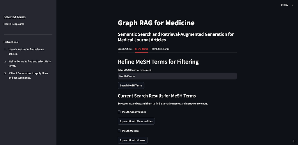
- Refine Terms: Second, the user decides the MeSH terms to use to filter the returned results. Since we also vectorized the MeSH terms, we can have the user enter a natural language prompt to get the most relevant MeSH terms. Then, we allow the user to expand these terms to see their alternative names and narrower concepts. The user can select as many terms as they want for their filter criteria.
- Filter & Summarize: Third, the user applies the selected terms as filters to the original ten journal articles. We can do this since the PubMed articles are tagged with MeSH terms. Finally, we let the user enter an additional prompt to send to the LLM along with the filtered journal articles. This is the generative step of the RAG app.
Let’s go through these steps one at a time. You can see the full app and code on my GitHub, but here is the structure:
-- app.py (a python file that drives the app and calls other functions as needed)
-- query_functions (a folder containing python files with queries)
  -- rdf_queries.py (python file with RDF queries)
  -- weaviate_queries.py (python file containing weaviate queries)
-- PubMedGraph.ttl (the pubmed data in RDF format, stored as a ttl file)
Search Articles
First, want to do is implement Weaviate’s vector similarity search. Since our articles are vectorized, we can send a search term to the vector database and get similar articles back.
The main function that searches for relevant journal articles in the vector database is in app.py:
# --- TAB 1: Search Articles ---
with tab_search:
    st.header("Search Articles (Vector Query)")
    query_text = st.text_input("Enter your vector search term (e.g., Mouth Neoplasms):", key="vector_search")

    if st.button("Search Articles", key="search_articles_btn"):
        try:
            client = initialize_weaviate_client()
            article_results = query_weaviate_articles(client, query_text)

            # Extract URIs here
            article_uris = [
                result["properties"].get("article_URI")
                for result in article_results
                if result["properties"].get("article_URI")
            ]

            # Store article_uris in the session state
            st.session_state.article_uris = article_uris

            st.session_state.article_results = [
                {
                    "Title": result["properties"].get("title", "N/A"),
                    "Abstract": (result["properties"].get("abstractText", "N/A")[:100] + "..."),
                    "Distance": result["distance"],
                    "MeSH Terms": ", ".join(
                        ast.literal_eval(result["properties"].get("meshMajor", "[]"))
                        if result["properties"].get("meshMajor") else []
                    ),

                }
                for result in article_results
            ]
            client.close()
        except Exception as e:
            st.error(f"Error during article search: {e}")

    if st.session_state.article_results:
        st.write("**Search Results for Articles:**")
        st.table(st.session_state.article_results)
    else:
        st.write("No articles found yet.")
This function uses the queries stored in weaviate_queries to establish the Weaviate client (initialize_weaviate_client) and search for articles (query_weaviate_articles). Then we display the returned articles in a table, along with their abstracts, distance (how close they are to the search term), and the MeSH terms that they are tagged with.
The function to query Weaviate in weaviate_queries.py looks like this:
# Function to query Weaviate for Articles
def query_weaviate_articles(client, query_text, limit=10):
    # Perform vector search on Article collection
    response = client.collections.get("Article").query.near_text(
        query=query_text,
        limit=limit,
        return_metadata=MetadataQuery(distance=True)
    )

    # Parse response
    results = []
    for obj in response.objects:
        results.append({
            "uuid": obj.uuid,
            "properties": obj.properties,
            "distance": obj.metadata.distance,
        })
    return results
As you can see, I put a limit of ten results here just to make it simpler, but you can change that. This is just using vector similarity search in Weaviate to return relevant results.
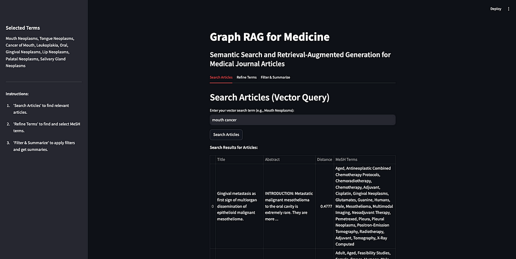
The end result in the app looks like this:
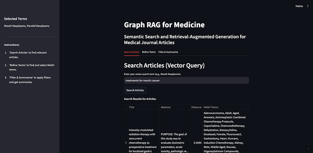
As a demo, I will search the term “treatments for mouth cancer”. As you can see, 10 articles are returned, mostly relevant. This demonstrates both the strengths and weaknesses of vector based retrieval.
The strength is that we can build a semantic search functionality on our data with minimal effort. As you can see above, all we did was set up the client and send the data to a vector database. Once our data has been vectorized, we can do semantic searches, similarity searches, and even RAG. I have put some of that in the notebook accompanying this post, but there’s a lot more in Weaviate’s official docs.
The weakness of vector based retrieval, as I mentioned above are that they are black-box and struggle with factual knowledge. In our example, it looks like most of the articles are about some kind of treatment or therapy for some kind of cancer. Some of the articles are about mouth cancer specifically, some are about a sub-type of mouth cancer like gingival cancer (cancer of the gums), and palatal cancer (cancer of the palate). But there are also articles about nasopharyngeal cancer (cancer of the upper throat), mandibular cancer (cancer of the jaw), and esophageal cancer (cancer of the esophagus). None of these (upper throat, jaw, or esophagus) are considered mouth cancer. It is understandable why an article about a specific cancer radiation therapy for nasopharyngeal neoplasms would be considered similar to the prompt “treatments for mouth cancer” but it may not be relevant if you are only looking for treatments for mouth cancer. If we were to plug these ten articles directly into our prompt to the LLM and ask it to “summarize the different treatment options,” we would be getting incorrect information.
The purpose of RAG is to give an LLM a very specific set of additional information to better answer your question — if that information is incorrect or irrelevant, it can lead to misleading responses from the LLM. This is often referred to as “context poisoning”. What is especially dangerous about context poisoning is that the response isn’t necessarily factually inaccurate (the LLM may accurately summarize the treatment options we feed it), and it isn’t necessarily based on an inaccurate piece of data (presumably the journal articles themselves are accurate), it’s just using the wrong data to answer your question. In this example, the user could be reading about how to treat the wrong kind of cancer, which seems very bad.
Refine Terms
KGs can help improve the accuracy of responses and reduce the likelihood of context poisoning by refining the results from the vector database. The next step is for selecting what MeSH terms we want to use to filter the articles. First, we do another vector similarity search against the vector database but on the Terms collection. This is because the user may not be familiar with the MeSH controlled vocabulary. In our example above, I searched for, “therapies for mouth cancer”, but “mouth cancer” is not a term in MeSH — they use “Mouth Neoplasms”. We want the user to be able to start exploring the MeSH terms without having a prior understanding of them — this is good practice regardless of the metadata used to tag the content.
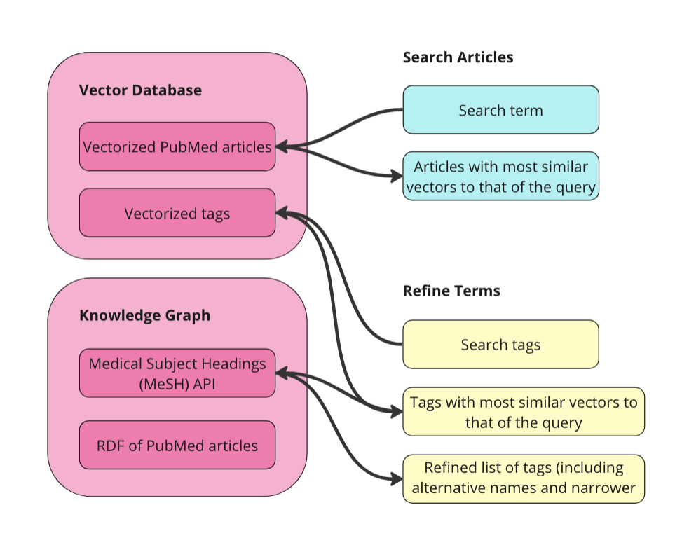
The function to get relevant MeSH terms is nearly identical to the previous Weaviate query. Just replace Article with term:
# Function to query Weaviate for MeSH Terms
def query_weaviate_terms(client, query_text, limit=10):
    # Perform vector search on MeshTerm collection
    response = client.collections.get("term").query.near_text(
        query=query_text,
        limit=limit,
        return_metadata=MetadataQuery(distance=True)
    )

    # Parse response
    results = []
    for obj in response.objects:
        results.append({
            "uuid": obj.uuid,
            "properties": obj.properties,
            "distance": obj.metadata.distance,
        })
    return results
Here is what it looks like in the app:
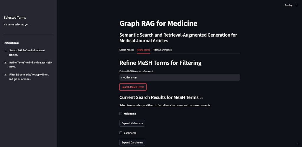
As you can see, I searched for “mouth cancer” and the most similar terms were returned. Mouth cancer was not returned, as that is not a term in MeSH, but Mouth Neoplasms is on the list.
The next step is to allow the user to expand the returned terms to see alternative names and narrower concepts. This requires querying the MeSH API. This was the trickiest part of this app for a number of reasons. The biggest problem is that Streamlit requires that everything has a unique ID but MeSH terms can repeat — if one of the returned concepts is a child of another, then when you expand the parent you will have a duplicate of the child. I think I took care of most of the big issues and the app should work, but there are probably bugs to find at this stage.
The functions we rely on are found in rdf_queries.py. We need one to get the alternative names for a term:
# Fetch alternative names and triples for a MeSH term
def get_concept_triples_for_term(term):
    term = sanitize_term(term)  # Sanitize input term
    sparql = SPARQLWrapper("https://id.nlm.nih.gov/mesh/sparql")
    query = f"""
    PREFIX rdf: <http://www.w3.org/1999/02/22-rdf-syntax-ns#>
    PREFIX rdfs: <http://www.w3.org/2000/01/rdf-schema#>
    PREFIX meshv: <http://id.nlm.nih.gov/mesh/vocab#>
    PREFIX mesh: <http://id.nlm.nih.gov/mesh/>

    SELECT ?subject ?p ?pLabel ?o ?oLabel
    FROM <http://id.nlm.nih.gov/mesh>
    WHERE {{
        ?subject rdfs:label "{term}"@en .
        ?subject ?p ?o .
        FILTER(CONTAINS(STR(?p), "concept"))
        OPTIONAL {{ ?p rdfs:label ?pLabel . }}
        OPTIONAL {{ ?o rdfs:label ?oLabel . }}
    }}
    """
    try:
        sparql.setQuery(query)
        sparql.setReturnFormat(JSON)
        results = sparql.query().convert()

        triples = set()
        for result in results["results"]["bindings"]:
            obj_label = result.get("oLabel", {}).get("value", "No label")
            triples.add(sanitize_term(obj_label))  # Sanitize term before adding

        # Add the sanitized term itself to ensure it's included
        triples.add(sanitize_term(term))
        return list(triples)

    except Exception as e:
        print(f"Error fetching concept triples for term '{term}': {e}")
        return []
We also need functions to get the narrower (child) concepts for a given term. I have two functions that achieve this — one that gets the immediate children of a term and one recursive function that returns all children of a given depth.
# Fetch narrower concepts for a MeSH term
def get_narrower_concepts_for_term(term):
    term = sanitize_term(term)  # Sanitize input term
    sparql = SPARQLWrapper("https://id.nlm.nih.gov/mesh/sparql")
    query = f"""
    PREFIX rdf: <http://www.w3.org/1999/02/22-rdf-syntax-ns#>
    PREFIX rdfs: <http://www.w3.org/2000/01/rdf-schema#>
    PREFIX meshv: <http://id.nlm.nih.gov/mesh/vocab#>
    PREFIX mesh: <http://id.nlm.nih.gov/mesh/>

    SELECT ?narrowerConcept ?narrowerConceptLabel
    WHERE {{
        ?broaderConcept rdfs:label "{term}"@en .
        ?narrowerConcept meshv:broaderDescriptor ?broaderConcept .
        ?narrowerConcept rdfs:label ?narrowerConceptLabel .
    }}
    """
    try:
        sparql.setQuery(query)
        sparql.setReturnFormat(JSON)
        results = sparql.query().convert()

        concepts = set()
        for result in results["results"]["bindings"]:
            subject_label = result.get("narrowerConceptLabel", {}).get("value", "No label")
            concepts.add(sanitize_term(subject_label))  # Sanitize term before adding

        return list(concepts)

    except Exception as e:
        print(f"Error fetching narrower concepts for term '{term}': {e}")
        return []

# Recursive function to fetch narrower concepts to a given depth
def get_all_narrower_concepts(term, depth=2, current_depth=1):
    term = sanitize_term(term)  # Sanitize input term
    all_concepts = {}
    try:
        narrower_concepts = get_narrower_concepts_for_term(term)
        all_concepts[sanitize_term(term)] = narrower_concepts

        if current_depth < depth:
            for concept in narrower_concepts:
                child_concepts = get_all_narrower_concepts(concept, depth, current_depth + 1)
                all_concepts.update(child_concepts)

    except Exception as e:
        print(f"Error fetching all narrower concepts for term '{term}': {e}")

    return all_concepts
The other important part of step 2 is to allow the user to select terms to add to a list of “Selected Terms”. These will appear in the sidebar on the left of the screen. There are a lot of things that can improve this step like:
- There is no way to clear all but you can clear the cache or refresh the browser if needed.
- There is no way to ‘select all narrower concepts’ which would be helpful.
- There is no option to add rules for filtering. Right now, we are just assuming that the article must contain term A OR term B OR term C etc. The rankings at the end are based on the number of terms the articles are tagged with.
Here is what it looks like in the app:
I can expand Mouth Neoplasms to see the alternative names, in this case, “Cancer of Mouth”, along with all of the narrower concepts. As you can see, most of the narrower concepts have their own children, which you can expand as well. For the purposes of this demo, I am going to select all children of Mouth Neoplasms.
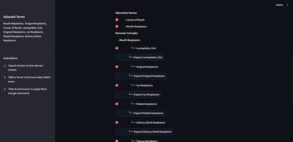
This step is important not just because it allows the user to filter the search results, but also because it is a way for the user to explore the MeSH graph itself and learn from it. For example, this would be the place for the user to learn that nasopharyngeal neoplasms are not a subset of mouth neoplasms.
Filter & Summarize
Now that you’ve got your articles and your filter terms, you can apply the filter and summarize the results. This is where we bring the original 10 articles returned in step one together with the refined list of MeSH terms. We allow the user to add additional context to the prompt before sending it to the LLM.
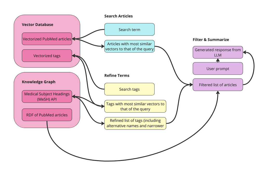
The way we do this filtering is that we need to get the URIs for the 10 articles from the original search. Then we can query our knowledge graph for which of those articles have been tagged with the associated MeSH terms. Additionally, we save the abstracts of these articles for use in the next step. This would be the place where we could filter based on access control or other user-controlled parameters like author, filetype, date published, etc. I didn’t include any of that in this app but I did add in properties for access control and date published in case we want to add that in this UI later.
Here is what the code looks like in app.py:
        if st.button("Filter Articles"):
            try:
                # Check if we have URIs from tab 1
                if "article_uris" in st.session_state and st.session_state.article_uris:
                    article_uris = st.session_state.article_uris

                    # Convert list of URIs into a string for the VALUES clause or FILTER
                    article_uris_string = ", ".join([f"<{str(uri)}>" for uri in article_uris])

                    SPARQL_QUERY = """
                    PREFIX schema: <http://schema.org/>
                    PREFIX ex: <http://example.org/>

                    SELECT ?article ?title ?abstract ?datePublished ?access ?meshTerm
                    WHERE {{
                      ?article a ex:Article ;
                               schema:name ?title ;
                               schema:description ?abstract ;
                               schema:datePublished ?datePublished ;
                               ex:access ?access ;
                               schema:about ?meshTerm .

                      ?meshTerm a ex:MeSHTerm .

                      FILTER (?article IN ({article_uris}))
                    }}
                    """
                    # Insert the article URIs into the query
                    query = SPARQL_QUERY.format(article_uris=article_uris_string)
                else:
                    st.write("No articles selected from Tab 1.")
                    st.stop()

                # Query the RDF and save results in session state
                top_articles = query_rdf(LOCAL_FILE_PATH, query, final_terms)
                st.session_state.filtered_articles = top_articles

                if top_articles:

                    # Combine abstracts from top articles and save in session state
                    def combine_abstracts(ranked_articles):
                        combined_text = " ".join(
                            [f"Title: {data['title']} Abstract: {data['abstract']}" for article_uri, data in
                             ranked_articles]
                        )
                        return combined_text


                    st.session_state.combined_text = combine_abstracts(top_articles)

                else:
                    st.write("No articles found for the selected terms.")
            except Exception as e:
                st.error(f"Error filtering articles: {e}")
This uses the function query_rdf in the rdf_queries.py file. That function looks like this:
# Function to query RDF using SPARQL
def query_rdf(local_file_path, query, mesh_terms, base_namespace="http://example.org/mesh/"):
    if not mesh_terms:
        raise ValueError("The list of MeSH terms is empty or invalid.")

    print("SPARQL Query:", query)

    # Create and parse the RDF graph
    g = Graph()
    g.parse(local_file_path, format="ttl")

    article_data = {}

    for term in mesh_terms:
        # Convert the term to a valid URI
        mesh_term_uri = convert_to_uri(term, base_namespace)
        #print("Term:", term, "URI:", mesh_term_uri)

        # Perform SPARQL query with initBindings
        results = g.query(query, initBindings={'meshTerm': mesh_term_uri})

        for row in results:
            article_uri = row['article']
            if article_uri not in article_data:
                article_data[article_uri] = {
                    'title': row['title'],
                    'abstract': row['abstract'],
                    'datePublished': row['datePublished'],
                    'access': row['access'],
                    'meshTerms': set()
                }
            article_data[article_uri]['meshTerms'].add(str(row['meshTerm']))
        #print("DEBUG article_data:", article_data)

    # Rank articles by the number of matching MeSH terms
    ranked_articles = sorted(
        article_data.items(),
        key=lambda item: len(item[1]['meshTerms']),
        reverse=True
    )
    return ranked_articles[:10]
As you can see, this function also converts the MeSH terms to URIs so we can filter using the graph. Be careful in the way you convert terms to URIs and ensure it aligns with the other functions.
Here is what it looks like in the app:
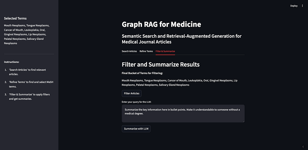
As you can see, the two MeSH terms we selected from the previous step are here. If I click “Filter Articles,” it will filter the original 10 articles using our filter criteria in step 2. The articles will be returned with their full abstracts, along with their tagged MeSH terms (see image below).
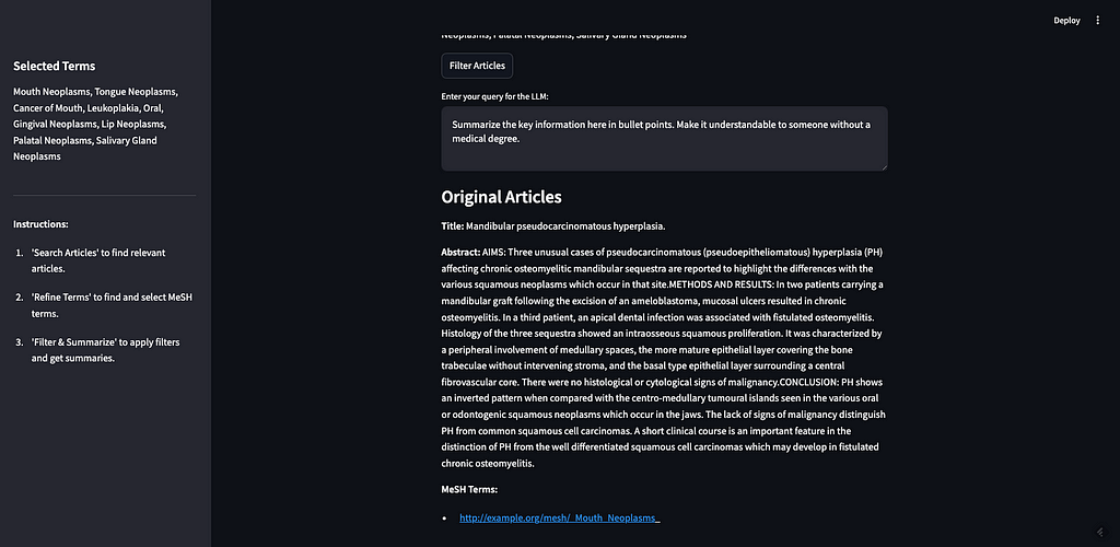
There are 5 articles returned. Two are tagged with “mouth neoplasms,” one with “gingival neoplasms,” and two with “palatal neoplasms”.
Now that we have a refined list of articles we want to use to generate a response, we can move to the final step. We want to send these articles to an LLM to generate a response but we can also add in additional context to the prompt. I have a default prompt that says, “Summarize the key information here in bullet points. Make it understandable to someone without a medical degree.” For this demo, I am going to adjust the prompt to reflect our original search term:

The results are as follows:
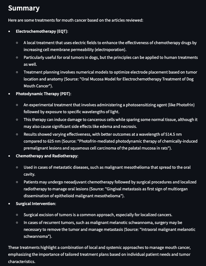
The results look better to me, mostly because I know that the articles we are summarizing are, presumably, about treatments for mouth cancer. The dataset doesn’t contain the actual journal articles, just the abstracts. So these results are just summaries of summaries. There may be some value to this, but if we were building a real app and not just a demo, this is the step where we could incorporate the full text of the articles. Alternatively, this is where the user/researcher would go read these articles themselves, rather than relying exclusively on the LLM for the summaries.
Conclusion
This tutorial demonstrates how combining vector databases and knowledge graphs can significantly enhance RAG applications. By leveraging vector similarity for initial searches and structured knowledge graph metadata for filtering and organization, we can build a system that delivers accurate, explainable, and domain-specific results. The integration of MeSH, a well-established controlled vocabulary, highlights the power of domain expertise in curating metadata, which ensures that the retrieval step aligns with the unique needs of the application while maintaining interoperability with other systems. This approach is not limited to medicine — its principles can be applied across domains wherever structured data and textual information coexist.
This tutorial underscores the importance of leveraging each technology for what it does best. Vector databases excel at similarity-based retrieval, while knowledge graphs shine in providing context, structure, and semantics. Additionally, scaling RAG applications demands a metadata layer to break down data silos and enforce governance policies. Thoughtful design, rooted in domain-specific metadata and robust governance, is the path to building RAG systems that are not only accurate but also scalable.
How to Build a Graph RAG App was originally published in Towards Data Science on Medium, where people are continuing the conversation by highlighting and responding to this story.
Image by AuthorUsing knowledge graphs and AI to retrieve, filter, and summarize medical journal articlesThe accompanying code for the app and notebook are here.Knowledge graphs (KGs) and Large Language Models (LLMs) are a match made in heaven. My previous posts discuss the complementarities of these two technologies in more detail but the short version is, “some of the main weaknesses of LLMs, that they are black-box models and struggle with factual knowledge, are some of KGs’ greatest strengths. KGs are, essentially, collections of facts, and they are fully interpretable.”This article is all about building a simple Graph RAG app. What is RAG? RAG, or Retrieval-Augmented Generation, is about retrieving relevant information to augment a prompt that is sent to an LLM, which generates a response. Graph RAG is RAG that uses a knowledge graph as part of the retrieval portion. If you’ve never heard of Graph RAG, or want a refresher, I’d watch this video.The basic idea is that, rather than sending your prompt directly to an LLM, which was not trained on your data, you can supplement your prompt with the relevant information needed for the LLM to answer your prompt accurately. The example I use often is copying a job description and my resume into ChatGPT to write a cover letter. The LLM is able to provide a much more relevant response to my prompt, ‘write me a cover letter,’ if I give it my resume and the description of the job I am applying for. Since knowledge graphs are built to store knowledge, they are a perfect way to store internal data and supplement LLM prompts with additional context, improving the accuracy and contextual understanding of the responses.This technology has many, many, applications such customer service bots, drug discovery, automated regulatory report generation in life sciences, talent acquisition and management for HR, legal research and writing, and wealth advisor assistants. Because of the wide applicability and the potential to improve the performance of LLM tools, Graph RAG (that’s the term I’ll use here) has been blowing up in popularity. Here is a graph showing interest over time based on Google searches.Source: https://trends.google.com/Graph RAG has experienced a surge in search interest, even surpassing terms like knowledge graphs and retrieval-augmented generation. Note that Google Trends measures relative search interest, not absolute number of searches. The spike in July 2024 for searches of Graph RAG coincides with the week Microsoft announced that their GraphRAG application would be available on GitHub.The excitement around Graph RAG is broader than just Microsoft, however. Samsung acquired RDFox, a knowledge graph company, in July of 2024. The article announcing that acquisition did not mention Graph RAG explicitly, but in this article in Forbes published in November 2024, a Samsung spokesperson stated, “We plan to develop knowledge graph technology, one of the main technologies of personalized AI, and organically connect with generated AI to support user-specific services.”In October 2024, Ontotext, a leading graph database company, and Semantic Web company, the maker of PoolParty, a knowledge graph curation platform, merged to form Graphwise. According to the press release, the merger aims to “democratize the evolution of Graph RAG as a category.”While some of the buzz around Graph RAG may come from the broader excitement surrounding chatbots and generative AI, it reflects a genuine evolution in how knowledge graphs are being applied to solve complex, real-world problems. One example is that LinkedIn applied Graph RAG to improve their customer service technical support. Because the tool was able to retrieve the relevant data (like previously solved similar tickets or questions) to feed the LLM, the responses were more accurate and the mean resolution time dropped from 40 hours to 15 hours.This post will go through the construction of a pretty simple, but I think illustrative, example of how Graph RAG can work in practice. The end result is an app that a non-technical user can interact with. Like my last post, I will use a dataset consisting of medical journal articles from PubMed. The idea is that this is an app that someone in the medical field could use to do literature review. The same principles can be applied to many use cases however, which is why Graph RAG is so exciting.The structure of the app, along with this post is as follows:Step zero is preparing the data. I will explain the details below but the overall goal is to vectorize the raw data and, separately, turn it into an RDF graph. As long as we keep URIs tied to the articles before we vectorize, we can navigate across a graph of articles and a vector space of articles. Then, we can:Search Articles: use the power of the vector database to do an initial search of relevant articles given a search term. I will use vector similarity to retrieve articles with the most similar vectors to that of the search term.Refine Terms: explore the Medical Subject Headings (MeSH) biomedical vocabulary to select terms to use to filter the articles from step 1. This controlled vocabulary contains medical terms, alternative names, narrower concepts, and many other properties and relationships.Filter & Summarize: use the MeSH terms to filter the articles to avoid ‘context poisoning’. Then send the remaining articles to an LLM along with an additional prompt like, “summarize in bullets.”Some notes on this app and tutorial before we get started:This set-up uses knowledge graphs exclusively for metadata. This is only possible because each article in my dataset has already been tagged with terms that are part of a rich controlled vocabulary. I am using the graph for structure and semantics and the vector database for similarity-based retrieval, ensuring each technology is used for what it does best. Vector similarity can tell us “esophageal cancer” is semantically similar to “mouth cancer”, but knowledge graphs can tell us the details of the relationship between “esophageal cancer” and “mouth cancer.”The data I used for this app is a collection of medical journal articles from PubMed (more on the data below). I chose this dataset because it is structured (tabular) but also contains text in the form of abstracts for each article, and because it is already tagged with topical terms that are aligned with a well-established controlled vocabulary (MeSH). Because these are medical articles, I have called this app ‘Graph RAG for Medicine.’ But this same structure can be applied to any domain and is not specific to the medical field.What I hope this tutorial and app demonstrate is that you can improve the results of your RAG application in terms of accuracy and explainability by incorporating a knowledge graph into the retrieval step. I will show how KGs can improve the accuracy of RAG applications in two ways: by giving the user a way of filtering the context to ensure the LLM is only being fed the most relevant information; and by using domain specific controlled vocabularies with dense relationships that are maintained and curated by domain experts to do the filtering.What this tutorial and app don’t directly showcase are two other significant ways KGs can enhance RAG applications: governance, access control, and regulatory compliance; and efficiency and scalability. For governance, KGs can do more than filter content for relevancy to improve accuracy — they can enforce data governance policies. For instance, if a user lacks permission to access certain content, that content can be excluded from their RAG pipeline. On the efficiency and scalability side, KGs can help ensure RAG applications don’t die on the shelf. While it’s easy to create an impressive one-off RAG app (that’s literally the purpose of this tutorial), many companies struggle with a proliferation of disconnected POCs that lack a cohesive framework, structure, or platform. That means many of those apps are not going to survive long. A metadata layer powered by KGs can break down data silos, providing the foundation needed to build, scale, and maintain RAG applications effectively. Using a rich controlled vocabulary like MeSH for the metadata tags on these articles is a way of ensuring this Graph RAG app can be integrated with other systems and reducing the risk that it becomes a silo.Step 0: Prepare the dataThe code to prepare the data is in this notebook.As mentioned, I’ve again decided to use this dataset of 50,000 research articles from the PubMed repository (License CC0: Public Domain). This dataset contains the title of the articles, their abstracts, as well as a field for metadata tags. These tags are from the Medical Subject Headings (MeSH) controlled vocabulary thesaurus. The PubMed articles are really just metadata on the articles — there are abstracts for each article but we don’t have the full text. The data is already in tabular format and tagged with MeSH terms.We can vectorize this tabular dataset directly. We could turn it into a graph (RDF) before we vectorize, but I didn’t do that for this app and I don’t know that it would help the final results for this kind of data. The most important thing about vectorizing the raw data is that we add Unique Resource Identifiers (URIs) to each article first. A URI is a unique ID for navigating RDF data and it is necessary for us to go back and forth between vectors and entities in our graph. Additionally, we will create a separate collection in our vector database for the MeSH terms. This will allow the user to search for relevant terms without having prior knowledge of this controlled vocabulary. Below is a diagram of what we are doing to prepare our data.Image by AuthorWe have two collections in our vector database to query: articles and terms. We also have the data represented as a graph in RDF format. Since MeSH has an API, I am just going to query the API directly to get alternative names and narrower concepts for terms.Vectorize data in WeaviateFirst import the required packages and set up the Weaviate client:import weaviatefrom weaviate.util import generate_uuid5from weaviate.classes.init import Authimport osimport jsonimport pandas as pdclient = weaviate.connect_to_weaviate_cloud( cluster_url=”XXX”, # Replace with your Weaviate Cloud URL auth_credentials=Auth.api_key(“XXX”), # Replace with your Weaviate Cloud key headers={‘X-OpenAI-Api-key’: “XXX”} # Replace with your OpenAI API key)Read in the PubMed journal articles. I am using Databricks to run this notebook so you may need to change this, depending on where you run it. The goal here is just to get the data into a pandas DataFrame.df = spark.sql(“SELECT * FROM workspace.default.pub_med_multi_label_text_classification_dataset_processed”).toPandas()If you’re running this locally, just do:df = pd.read_csv(“PubMed Multi Label Text Classification Dataset Processed.csv”)Then clean the data up a bit:import numpy as np# Replace infinity values with NaN and then fill NaN valuesdf.replace([np.inf, -np.inf], np.nan, inplace=True)df.fillna(”, inplace=True)# Convert columns to string typedf[‘Title’] = df[‘Title’].astype(str)df[‘abstractText’] = df[‘abstractText’].astype(str)df[‘meshMajor’] = df[‘meshMajor’].astype(str)Now we need to create a URI for each article and add that in as a new column. This is important because the URI is the way we can connect the vector representation of an article with the knowledge graph representation of the article.import urllib.parsefrom rdflib import Graph, RDF, RDFS, Namespace, URIRef, Literal# Function to create a valid URIdef create_valid_uri(base_uri, text): if pd.isna(text): return None # Encode text to be used in URI sanitized_text = urllib.parse.quote(text.strip().replace(‘ ‘, ‘_’).replace(‘”‘, ”).replace(‘<‘, ”).replace(‘>’, ”).replace(“‘”, “_”)) return URIRef(f”{base_uri}/{sanitized_text}”)# Function to create a valid URI for Articlesdef create_article_uri(title, base_namespace=”http://example.org/article/”): “”” Creates a URI for an article by replacing non-word characters with underscores and URL-encoding. Args: title (str): The title of the article. base_namespace (str): The base namespace for the article URI. Returns: URIRef: The formatted article URI. “”” if pd.isna(title): return None # Replace non-word characters with underscores sanitized_title = re.sub(r’W+’, ‘_’, title.strip()) # Condense multiple underscores into a single underscore sanitized_title = re.sub(r’_+’, ‘_’, sanitized_title) # URL-encode the term encoded_title = quote(sanitized_title) # Concatenate with base_namespace without adding underscores uri = f”{base_namespace}{encoded_title}” return URIRef(uri)# Add a new column to the DataFrame for the article URIsdf[‘Article_URI’] = df[‘Title’].apply(lambda title: create_valid_uri(“http://example.org/article”, title))We also want to create a DataFrame of all of the MeSH terms that are used to tag the articles. This will be helpful later when we want to search for similar MeSH terms.# Function to clean and parse MeSH termsdef parse_mesh_terms(mesh_list): if pd.isna(mesh_list): return [] return [ term.strip().replace(‘ ‘, ‘_’) for term in mesh_list.strip(“[]'”).split(‘,’) ]# Function to create a valid URI for MeSH termsdef create_valid_uri(base_uri, text): if pd.isna(text): return None sanitized_text = urllib.parse.quote( text.strip() .replace(‘ ‘, ‘_’) .replace(‘”‘, ”) .replace(‘<‘, ”) .replace(‘>’, ”) .replace(“‘”, “_”) ) return f”{base_uri}/{sanitized_text}”# Extract and process all MeSH termsall_mesh_terms = []for mesh_list in df[“meshMajor”]: all_mesh_terms.extend(parse_mesh_terms(mesh_list))# Deduplicate termsunique_mesh_terms = list(set(all_mesh_terms))# Create a DataFrame of MeSH terms and their URIsmesh_df = pd.DataFrame({ “meshTerm”: unique_mesh_terms, “URI”: [create_valid_uri(“http://example.org/mesh”, term) for term in unique_mesh_terms]})# Display the DataFrameprint(mesh_df)Vectorize the articles DataFrame:from weaviate.classes.config import Configure#define the collectionarticles = client.collections.create( name = “Article”, vectorizer_config=Configure.Vectorizer.text2vec_openai(), # If set to “none” you must always provide vectors yourself. Could be any other “text2vec-*” also. generative_config=Configure.Generative.openai(), # Ensure the `generative-openai` module is used for generative queries)#add ojectsarticles = client.collections.get(“Article”)with articles.batch.dynamic() as batch: for index, row in df.iterrows(): batch.add_object({ “title”: row[“Title”], “abstractText”: row[“abstractText”], “Article_URI”: row[“Article_URI”], “meshMajor”: row[“meshMajor”], })Now vectorize the MeSH terms:#define the collectionterms = client.collections.create( name = “term”, vectorizer_config=Configure.Vectorizer.text2vec_openai(), # If set to “none” you must always provide vectors yourself. Could be any other “text2vec-*” also. generative_config=Configure.Generative.openai(), # Ensure the `generative-openai` module is used for generative queries)#add ojectsterms = client.collections.get(“term”)with terms.batch.dynamic() as batch: for index, row in mesh_df.iterrows(): batch.add_object({ “meshTerm”: row[“meshTerm”], “URI”: row[“URI”], })You can, at this point, run semantic search, similarity search, and RAG directly against the vectorized dataset. I won’t go through all of that here but you can look at the code in my accompanying notebook to do that.Turn data into a knowledge graphI am just using the same code we used in the last post to do this. We are basically turning every row in the data into an “Article” entity in our KG. Then we are giving each of these articles properties for title, abstract, and MeSH terms. We are also turning every MeSH term into an entity as well. This code also adds random dates to each article for a property called date published and a random number between 1 and 10 to a property called access. We won’t use those properties in this demo. Below is a visual representation of the graph we are creating from the data.Image by AuthorHere is how to iterate through the DataFrame and turn it into RDF data:from rdflib import Graph, RDF, RDFS, Namespace, URIRef, Literalfrom rdflib.namespace import SKOS, XSDimport pandas as pdimport urllib.parseimport randomfrom datetime import datetime, timedeltaimport refrom urllib.parse import quote# — Initialization —g = Graph()# Define namespacesschema = Namespace(‘http://schema.org/’)ex = Namespace(‘http://example.org/’)prefixes = { ‘schema’: schema, ‘ex’: ex, ‘skos’: SKOS, ‘xsd’: XSD}for p, ns in prefixes.items(): g.bind(p, ns)# Define classes and propertiesArticle = URIRef(ex.Article)MeSHTerm = URIRef(ex.MeSHTerm)g.add((Article, RDF.type, RDFS.Class))g.add((MeSHTerm, RDF.type, RDFS.Class))title = URIRef(schema.name)abstract = URIRef(schema.description)date_published = URIRef(schema.datePublished)access = URIRef(ex.access)g.add((title, RDF.type, RDF.Property))g.add((abstract, RDF.type, RDF.Property))g.add((date_published, RDF.type, RDF.Property))g.add((access, RDF.type, RDF.Property))# Function to clean and parse MeSH termsdef parse_mesh_terms(mesh_list): if pd.isna(mesh_list): return [] return [term.strip() for term in mesh_list.strip(“[]'”).split(‘,’)]# Enhanced convert_to_uri functiondef convert_to_uri(term, base_namespace=”http://example.org/mesh/”): “”” Converts a MeSH term into a standardized URI by replacing spaces and special characters with underscores, ensuring it starts and ends with a single underscore, and URL-encoding the term. Args: term (str): The MeSH term to convert. base_namespace (str): The base namespace for the URI. Returns: URIRef: The formatted URI. “”” if pd.isna(term): return None # Handle NaN or None terms gracefully # Step 1: Strip existing leading and trailing non-word characters (including underscores) stripped_term = re.sub(r’^W+|W+$’, ”, term) # Step 2: Replace non-word characters with underscores (one or more) formatted_term = re.sub(r’W+’, ‘_’, stripped_term) # Step 3: Replace multiple consecutive underscores with a single underscore formatted_term = re.sub(r’_+’, ‘_’, formatted_term) # Step 4: URL-encode the term to handle any remaining special characters encoded_term = quote(formatted_term) # Step 5: Add single leading and trailing underscores term_with_underscores = f”_{encoded_term}_” # Step 6: Concatenate with base_namespace without adding an extra underscore uri = f”{base_namespace}{term_with_underscores}” return URIRef(uri)# Function to generate a random date within the last 5 yearsdef generate_random_date(): start_date = datetime.now() – timedelta(days=5*365) random_days = random.randint(0, 5*365) return start_date + timedelta(days=random_days)# Function to generate a random access value between 1 and 10def generate_random_access(): return random.randint(1, 10)# Function to create a valid URI for Articlesdef create_article_uri(title, base_namespace=”http://example.org/article”): “”” Creates a URI for an article by replacing non-word characters with underscores and URL-encoding. Args: title (str): The title of the article. base_namespace (str): The base namespace for the article URI. Returns: URIRef: The formatted article URI. “”” if pd.isna(title): return None # Encode text to be used in URI sanitized_text = urllib.parse.quote(title.strip().replace(‘ ‘, ‘_’).replace(‘”‘, ”).replace(‘<‘, ”).replace(‘>’, ”).replace(“‘”, “_”)) return URIRef(f”{base_namespace}/{sanitized_text}”)# Loop through each row in the DataFrame and create RDF triplesfor index, row in df.iterrows(): article_uri = create_article_uri(row[‘Title’]) if article_uri is None: continue # Add Article instance g.add((article_uri, RDF.type, Article)) g.add((article_uri, title, Literal(row[‘Title’], datatype=XSD.string))) g.add((article_uri, abstract, Literal(row[‘abstractText’], datatype=XSD.string))) # Add random datePublished and access random_date = generate_random_date() random_access = generate_random_access() g.add((article_uri, date_published, Literal(random_date.date(), datatype=XSD.date))) g.add((article_uri, access, Literal(random_access, datatype=XSD.integer))) # Add MeSH Terms mesh_terms = parse_mesh_terms(row[‘meshMajor’]) for term in mesh_terms: term_uri = convert_to_uri(term, base_namespace=”http://example.org/mesh/”) if term_uri is None: continue # Add MeSH Term instance g.add((term_uri, RDF.type, MeSHTerm)) g.add((term_uri, RDFS.label, Literal(term.replace(‘_’, ‘ ‘), datatype=XSD.string))) # Link Article to MeSH Term g.add((article_uri, schema.about, term_uri))# Path to save the filefile_path = “/Workspace/PubMedGraph.ttl”# Save the fileg.serialize(destination=file_path, format=’turtle’)print(f”File saved at {file_path}”)OK, so now we have a vectorized version of the data, and a graph (RDF) version of the data. Each vector has a URI associated with it, which corresponds to an entity in the KG, so we can go back and forth between the data formats.Build an appI decided to use Streamlit to build the interface for this graph RAG app. Similar to the last blog post, I have kept the user flow the same.Search Articles: First, the user searches for articles using a search term. This relies exclusively on the vector database. The user’s search term(s) is sent to the vector database and the ten articles nearest the term in vector space are returned.Refine Terms: Second, the user decides the MeSH terms to use to filter the returned results. Since we also vectorized the MeSH terms, we can have the user enter a natural language prompt to get the most relevant MeSH terms. Then, we allow the user to expand these terms to see their alternative names and narrower concepts. The user can select as many terms as they want for their filter criteria.Filter & Summarize: Third, the user applies the selected terms as filters to the original ten journal articles. We can do this since the PubMed articles are tagged with MeSH terms. Finally, we let the user enter an additional prompt to send to the LLM along with the filtered journal articles. This is the generative step of the RAG app.Let’s go through these steps one at a time. You can see the full app and code on my GitHub, but here is the structure:– app.py (a python file that drives the app and calls other functions as needed)– query_functions (a folder containing python files with queries) — rdf_queries.py (python file with RDF queries) — weaviate_queries.py (python file containing weaviate queries)– PubMedGraph.ttl (the pubmed data in RDF format, stored as a ttl file)Search ArticlesFirst, want to do is implement Weaviate’s vector similarity search. Since our articles are vectorized, we can send a search term to the vector database and get similar articles back.Image by AuthorThe main function that searches for relevant journal articles in the vector database is in app.py:# — TAB 1: Search Articles —with tab_search: st.header(“Search Articles (Vector Query)”) query_text = st.text_input(“Enter your vector search term (e.g., Mouth Neoplasms):”, key=”vector_search”) if st.button(“Search Articles”, key=”search_articles_btn”): try: client = initialize_weaviate_client() article_results = query_weaviate_articles(client, query_text) # Extract URIs here article_uris = [ result[“properties”].get(“article_URI”) for result in article_results if result[“properties”].get(“article_URI”) ] # Store article_uris in the session state st.session_state.article_uris = article_uris st.session_state.article_results = [ { “Title”: result[“properties”].get(“title”, “N/A”), “Abstract”: (result[“properties”].get(“abstractText”, “N/A”)[:100] + “…”), “Distance”: result[“distance”], “MeSH Terms”: “, “.join( ast.literal_eval(result[“properties”].get(“meshMajor”, “[]”)) if result[“properties”].get(“meshMajor”) else [] ), } for result in article_results ] client.close() except Exception as e: st.error(f”Error during article search: {e}”) if st.session_state.article_results: st.write(“**Search Results for Articles:**”) st.table(st.session_state.article_results) else: st.write(“No articles found yet.”)This function uses the queries stored in weaviate_queries to establish the Weaviate client (initialize_weaviate_client) and search for articles (query_weaviate_articles). Then we display the returned articles in a table, along with their abstracts, distance (how close they are to the search term), and the MeSH terms that they are tagged with.The function to query Weaviate in weaviate_queries.py looks like this:# Function to query Weaviate for Articlesdef query_weaviate_articles(client, query_text, limit=10): # Perform vector search on Article collection response = client.collections.get(“Article”).query.near_text( query=query_text, limit=limit, return_metadata=MetadataQuery(distance=True) ) # Parse response results = [] for obj in response.objects: results.append({ “uuid”: obj.uuid, “properties”: obj.properties, “distance”: obj.metadata.distance, }) return resultsAs you can see, I put a limit of ten results here just to make it simpler, but you can change that. This is just using vector similarity search in Weaviate to return relevant results.The end result in the app looks like this:Image by AuthorAs a demo, I will search the term “treatments for mouth cancer”. As you can see, 10 articles are returned, mostly relevant. This demonstrates both the strengths and weaknesses of vector based retrieval.The strength is that we can build a semantic search functionality on our data with minimal effort. As you can see above, all we did was set up the client and send the data to a vector database. Once our data has been vectorized, we can do semantic searches, similarity searches, and even RAG. I have put some of that in the notebook accompanying this post, but there’s a lot more in Weaviate’s official docs.The weakness of vector based retrieval, as I mentioned above are that they are black-box and struggle with factual knowledge. In our example, it looks like most of the articles are about some kind of treatment or therapy for some kind of cancer. Some of the articles are about mouth cancer specifically, some are about a sub-type of mouth cancer like gingival cancer (cancer of the gums), and palatal cancer (cancer of the palate). But there are also articles about nasopharyngeal cancer (cancer of the upper throat), mandibular cancer (cancer of the jaw), and esophageal cancer (cancer of the esophagus). None of these (upper throat, jaw, or esophagus) are considered mouth cancer. It is understandable why an article about a specific cancer radiation therapy for nasopharyngeal neoplasms would be considered similar to the prompt “treatments for mouth cancer” but it may not be relevant if you are only looking for treatments for mouth cancer. If we were to plug these ten articles directly into our prompt to the LLM and ask it to “summarize the different treatment options,” we would be getting incorrect information.The purpose of RAG is to give an LLM a very specific set of additional information to better answer your question — if that information is incorrect or irrelevant, it can lead to misleading responses from the LLM. This is often referred to as “context poisoning”. What is especially dangerous about context poisoning is that the response isn’t necessarily factually inaccurate (the LLM may accurately summarize the treatment options we feed it), and it isn’t necessarily based on an inaccurate piece of data (presumably the journal articles themselves are accurate), it’s just using the wrong data to answer your question. In this example, the user could be reading about how to treat the wrong kind of cancer, which seems very bad.Refine TermsKGs can help improve the accuracy of responses and reduce the likelihood of context poisoning by refining the results from the vector database. The next step is for selecting what MeSH terms we want to use to filter the articles. First, we do another vector similarity search against the vector database but on the Terms collection. This is because the user may not be familiar with the MeSH controlled vocabulary. In our example above, I searched for, “therapies for mouth cancer”, but “mouth cancer” is not a term in MeSH — they use “Mouth Neoplasms”. We want the user to be able to start exploring the MeSH terms without having a prior understanding of them — this is good practice regardless of the metadata used to tag the content.Image by AuthorThe function to get relevant MeSH terms is nearly identical to the previous Weaviate query. Just replace Article with term:# Function to query Weaviate for MeSH Termsdef query_weaviate_terms(client, query_text, limit=10): # Perform vector search on MeshTerm collection response = client.collections.get(“term”).query.near_text( query=query_text, limit=limit, return_metadata=MetadataQuery(distance=True) ) # Parse response results = [] for obj in response.objects: results.append({ “uuid”: obj.uuid, “properties”: obj.properties, “distance”: obj.metadata.distance, }) return resultsHere is what it looks like in the app:Image by AuthorAs you can see, I searched for “mouth cancer” and the most similar terms were returned. Mouth cancer was not returned, as that is not a term in MeSH, but Mouth Neoplasms is on the list.The next step is to allow the user to expand the returned terms to see alternative names and narrower concepts. This requires querying the MeSH API. This was the trickiest part of this app for a number of reasons. The biggest problem is that Streamlit requires that everything has a unique ID but MeSH terms can repeat — if one of the returned concepts is a child of another, then when you expand the parent you will have a duplicate of the child. I think I took care of most of the big issues and the app should work, but there are probably bugs to find at this stage.The functions we rely on are found in rdf_queries.py. We need one to get the alternative names for a term:# Fetch alternative names and triples for a MeSH termdef get_concept_triples_for_term(term): term = sanitize_term(term) # Sanitize input term sparql = SPARQLWrapper(“https://id.nlm.nih.gov/mesh/sparql”) query = f””” PREFIX rdf: <http://www.w3.org/1999/02/22-rdf-syntax-ns#> PREFIX rdfs: <http://www.w3.org/2000/01/rdf-schema#> PREFIX meshv: <http://id.nlm.nih.gov/mesh/vocab#> PREFIX mesh: <http://id.nlm.nih.gov/mesh/> SELECT ?subject ?p ?pLabel ?o ?oLabel FROM <http://id.nlm.nih.gov/mesh> WHERE {{ ?subject rdfs:label “{term}”@en . ?subject ?p ?o . FILTER(CONTAINS(STR(?p), “concept”)) OPTIONAL {{ ?p rdfs:label ?pLabel . }} OPTIONAL {{ ?o rdfs:label ?oLabel . }} }} “”” try: sparql.setQuery(query) sparql.setReturnFormat(JSON) results = sparql.query().convert() triples = set() for result in results[“results”][“bindings”]: obj_label = result.get(“oLabel”, {}).get(“value”, “No label”) triples.add(sanitize_term(obj_label)) # Sanitize term before adding # Add the sanitized term itself to ensure it’s included triples.add(sanitize_term(term)) return list(triples) except Exception as e: print(f”Error fetching concept triples for term ‘{term}’: {e}”) return []We also need functions to get the narrower (child) concepts for a given term. I have two functions that achieve this — one that gets the immediate children of a term and one recursive function that returns all children of a given depth.# Fetch narrower concepts for a MeSH termdef get_narrower_concepts_for_term(term): term = sanitize_term(term) # Sanitize input term sparql = SPARQLWrapper(“https://id.nlm.nih.gov/mesh/sparql”) query = f””” PREFIX rdf: <http://www.w3.org/1999/02/22-rdf-syntax-ns#> PREFIX rdfs: <http://www.w3.org/2000/01/rdf-schema#> PREFIX meshv: <http://id.nlm.nih.gov/mesh/vocab#> PREFIX mesh: <http://id.nlm.nih.gov/mesh/> SELECT ?narrowerConcept ?narrowerConceptLabel WHERE {{ ?broaderConcept rdfs:label “{term}”@en . ?narrowerConcept meshv:broaderDescriptor ?broaderConcept . ?narrowerConcept rdfs:label ?narrowerConceptLabel . }} “”” try: sparql.setQuery(query) sparql.setReturnFormat(JSON) results = sparql.query().convert() concepts = set() for result in results[“results”][“bindings”]: subject_label = result.get(“narrowerConceptLabel”, {}).get(“value”, “No label”) concepts.add(sanitize_term(subject_label)) # Sanitize term before adding return list(concepts) except Exception as e: print(f”Error fetching narrower concepts for term ‘{term}’: {e}”) return []# Recursive function to fetch narrower concepts to a given depthdef get_all_narrower_concepts(term, depth=2, current_depth=1): term = sanitize_term(term) # Sanitize input term all_concepts = {} try: narrower_concepts = get_narrower_concepts_for_term(term) all_concepts[sanitize_term(term)] = narrower_concepts if current_depth < depth: for concept in narrower_concepts: child_concepts = get_all_narrower_concepts(concept, depth, current_depth + 1) all_concepts.update(child_concepts) except Exception as e: print(f”Error fetching all narrower concepts for term ‘{term}’: {e}”) return all_conceptsThe other important part of step 2 is to allow the user to select terms to add to a list of “Selected Terms”. These will appear in the sidebar on the left of the screen. There are a lot of things that can improve this step like:There is no way to clear all but you can clear the cache or refresh the browser if needed.There is no way to ‘select all narrower concepts’ which would be helpful.There is no option to add rules for filtering. Right now, we are just assuming that the article must contain term A OR term B OR term C etc. The rankings at the end are based on the number of terms the articles are tagged with.Here is what it looks like in the app:Image by AuthorI can expand Mouth Neoplasms to see the alternative names, in this case, “Cancer of Mouth”, along with all of the narrower concepts. As you can see, most of the narrower concepts have their own children, which you can expand as well. For the purposes of this demo, I am going to select all children of Mouth Neoplasms.Image by AuthorThis step is important not just because it allows the user to filter the search results, but also because it is a way for the user to explore the MeSH graph itself and learn from it. For example, this would be the place for the user to learn that nasopharyngeal neoplasms are not a subset of mouth neoplasms.Filter & SummarizeNow that you’ve got your articles and your filter terms, you can apply the filter and summarize the results. This is where we bring the original 10 articles returned in step one together with the refined list of MeSH terms. We allow the user to add additional context to the prompt before sending it to the LLM.Image by AuthorThe way we do this filtering is that we need to get the URIs for the 10 articles from the original search. Then we can query our knowledge graph for which of those articles have been tagged with the associated MeSH terms. Additionally, we save the abstracts of these articles for use in the next step. This would be the place where we could filter based on access control or other user-controlled parameters like author, filetype, date published, etc. I didn’t include any of that in this app but I did add in properties for access control and date published in case we want to add that in this UI later.Here is what the code looks like in app.py: if st.button(“Filter Articles”): try: # Check if we have URIs from tab 1 if “article_uris” in st.session_state and st.session_state.article_uris: article_uris = st.session_state.article_uris # Convert list of URIs into a string for the VALUES clause or FILTER article_uris_string = “, “.join([f”<{str(uri)}>” for uri in article_uris]) SPARQL_QUERY = “”” PREFIX schema: <http://schema.org/> PREFIX ex: <http://example.org/> SELECT ?article ?title ?abstract ?datePublished ?access ?meshTerm WHERE {{ ?article a ex:Article ; schema:name ?title ; schema:description ?abstract ; schema:datePublished ?datePublished ; ex:access ?access ; schema:about ?meshTerm . ?meshTerm a ex:MeSHTerm . FILTER (?article IN ({article_uris})) }} “”” # Insert the article URIs into the query query = SPARQL_QUERY.format(article_uris=article_uris_string) else: st.write(“No articles selected from Tab 1.”) st.stop() # Query the RDF and save results in session state top_articles = query_rdf(LOCAL_FILE_PATH, query, final_terms) st.session_state.filtered_articles = top_articles if top_articles: # Combine abstracts from top articles and save in session state def combine_abstracts(ranked_articles): combined_text = ” “.join( [f”Title: {data[‘title’]} Abstract: {data[‘abstract’]}” for article_uri, data in ranked_articles] ) return combined_text st.session_state.combined_text = combine_abstracts(top_articles) else: st.write(“No articles found for the selected terms.”) except Exception as e: st.error(f”Error filtering articles: {e}”)This uses the function query_rdf in the rdf_queries.py file. That function looks like this:# Function to query RDF using SPARQLdef query_rdf(local_file_path, query, mesh_terms, base_namespace=”http://example.org/mesh/”): if not mesh_terms: raise ValueError(“The list of MeSH terms is empty or invalid.”) print(“SPARQL Query:”, query) # Create and parse the RDF graph g = Graph() g.parse(local_file_path, format=”ttl”) article_data = {} for term in mesh_terms: # Convert the term to a valid URI mesh_term_uri = convert_to_uri(term, base_namespace) #print(“Term:”, term, “URI:”, mesh_term_uri) # Perform SPARQL query with initBindings results = g.query(query, initBindings={‘meshTerm’: mesh_term_uri}) for row in results: article_uri = row[‘article’] if article_uri not in article_data: article_data[article_uri] = { ‘title’: row[‘title’], ‘abstract’: row[‘abstract’], ‘datePublished’: row[‘datePublished’], ‘access’: row[‘access’], ‘meshTerms’: set() } article_data[article_uri][‘meshTerms’].add(str(row[‘meshTerm’])) #print(“DEBUG article_data:”, article_data) # Rank articles by the number of matching MeSH terms ranked_articles = sorted( article_data.items(), key=lambda item: len(item[1][‘meshTerms’]), reverse=True ) return ranked_articles[:10]As you can see, this function also converts the MeSH terms to URIs so we can filter using the graph. Be careful in the way you convert terms to URIs and ensure it aligns with the other functions.Here is what it looks like in the app:Image by AuthorAs you can see, the two MeSH terms we selected from the previous step are here. If I click “Filter Articles,” it will filter the original 10 articles using our filter criteria in step 2. The articles will be returned with their full abstracts, along with their tagged MeSH terms (see image below).Image by AuthorThere are 5 articles returned. Two are tagged with “mouth neoplasms,” one with “gingival neoplasms,” and two with “palatal neoplasms”.Now that we have a refined list of articles we want to use to generate a response, we can move to the final step. We want to send these articles to an LLM to generate a response but we can also add in additional context to the prompt. I have a default prompt that says, “Summarize the key information here in bullet points. Make it understandable to someone without a medical degree.” For this demo, I am going to adjust the prompt to reflect our original search term:The results are as follows:The results look better to me, mostly because I know that the articles we are summarizing are, presumably, about treatments for mouth cancer. The dataset doesn’t contain the actual journal articles, just the abstracts. So these results are just summaries of summaries. There may be some value to this, but if we were building a real app and not just a demo, this is the step where we could incorporate the full text of the articles. Alternatively, this is where the user/researcher would go read these articles themselves, rather than relying exclusively on the LLM for the summaries.ConclusionThis tutorial demonstrates how combining vector databases and knowledge graphs can significantly enhance RAG applications. By leveraging vector similarity for initial searches and structured knowledge graph metadata for filtering and organization, we can build a system that delivers accurate, explainable, and domain-specific results. The integration of MeSH, a well-established controlled vocabulary, highlights the power of domain expertise in curating metadata, which ensures that the retrieval step aligns with the unique needs of the application while maintaining interoperability with other systems. This approach is not limited to medicine — its principles can be applied across domains wherever structured data and textual information coexist.This tutorial underscores the importance of leveraging each technology for what it does best. Vector databases excel at similarity-based retrieval, while knowledge graphs shine in providing context, structure, and semantics. Additionally, scaling RAG applications demands a metadata layer to break down data silos and enforce governance policies. Thoughtful design, rooted in domain-specific metadata and robust governance, is the path to building RAG systems that are not only accurate but also scalable.How to Build a Graph RAG App was originally published in Towards Data Science on Medium, where people are continuing the conversation by highlighting and responding to this story. knowledge-graph, graph, genai, llm, hands-on-tutorials Towards Data Science – MediumRead More

 Add to favorites


0 Comments