Understanding the theory and implementation of SAC RL in the context of Bioengineering

Introduction

The research domain of Reinforcement Learning (RL) has evolved greatly over the past years. The use of deep reinforcement learning methods such as Proximal Policy Optimisation (PPO) (Schulman, 2017) and Deep Deterministic Policy Gradient (DDPG) (Lillicrap, 2015) have enabled agents to solve tasks in high-dimensional environments. However, many of these model-free RL algorithms have struggled with stability during the training process. These challenges arise due to the brittle convergence properties, high variance in gradient estimation, very high sample complexity, and the sensitivity to hyperparameters in continuous action spaces. Given these problems, it is imperative to consider a newly devised RL algorithm that avoids such issues and expands applicability to complex, real-world problems. This new algorithm is the Soft Actor-Critic (SAC) deep RL network. (Haarnoja, 2018)

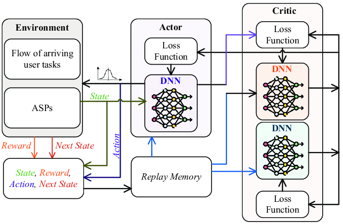
SAC is an off-policy Actor-Critic deep RL algorithm which is designed to address the stability and efficiency constraints of its predecessors. The SAC algorithm is based on the maximum entropy RL framework which aims for the actor part of the network to maximise the expected reward, while maximising entropy. It combines off-policy updates with a more stable formulation of the stochastic Actor-Critic method. An off-policy algorithm enables faster learning and better sample efficiency using experience replay, unlike on-policy methods such as PPO, which require new samples for each gradient step. For on-policy methods such as PPO, for each gradient step in the learning process, new samples must be collected. The aim of using stochastic policies and maximising entropy comes to promote the robustness and exploration of the algorithm by encouraging more randomness in the actions. Additionally, unlike PPO and DDPG, SAC uses twin Q-networks with a separate Actor network and entropy tuning to improve the stability and convergence when combining off-policy learning with high dimensional, nonlinear function approximation.

Off-policy RL methods have had a wide impact on bioengineering systems that improve patient lives. More specifically, RL has been applied to domains such as robotic arm control, drug delivery methods and most notably de novo drug design. (Svensson, 2024) Svensson et al. has used a number of on- and off-policy frameworks and different variants of replay buffers to learn a RNN-based molecule generation policy, to be active against DRD2 (a dopamine receptor). The paper realises that using experience replay across the board for high, intermediate and low scoring molecules has shown effects in improving the structural diversity and the number of active molecules generated. Replay buffers improve sample efficiency in training agents. They also reported that the use of off-policy methods and more specifically SAC, helps in promoting structural diversity by preventing mode collapse.

Theoretical Explanation

SAC uses ‘soft’ value functions by introducing the objective function with an entropy term, Η(π(a|s)). Accordingly, the network seeks to maximise both the expected return of lifetime rewards and the entropy of the policy. The entropy of the policy is defined as the unpredictability of a random variable, which increases with the range of possible values. Thus, the new entropy regularised objective becomes:

α is the temperature parameter that balances between exploration and exploitation.

In the implementation of soft value functions, we aim to maximise the entropy as the algorithm would assign equal probabilities to actions that have a similar Q-value. Maximising entropy also helps with preventing the agent from choosing actions that exploit inconsistencies in approximated Q-values. We can finally understand how SAC improves brittleness by allowing the network to explore more and not assign very high probabilities to one range of actions. This part is inspired by Vaishak V.Kumar’s explanation of the entropy maximisation in “Soft Actor-Critic Demystified”.

The SAC paper authors discuss that since the state value function approximates the soft value, there is really no essential need to train separate function approximators for the policy, since they relate to the state value according to the following equation. However, training three separate approximators provided better convergence.

The three function approximator networks are characterised as follows:

• Policy Network (Actor): the stochastic policy outputs a set of actions sampled from a Gaussian distribution. The policy parameters are learned by minimising the Kullback-Leibler Divergence as provided in this equation:

The KL-divergence compares the relative entropy or the difference between two probability distributions. So, in the equation, we are trying to minimise the difference between the distributions of the policy function and the exponentiated Q-function normalised by a function Z. Since the target density function is the Q-function, which is differentiable, we apply a reparametrisation trick on the policy to reduce the estimation of the variance.

ϵₜ is a vector sampled from a Gaussian distribution which describes the noise.

The policy objective is then updated to the following expression:

The policy objective is optimised using the following gradient estimation:

• Q-Network (Critic): includes two Q-value networks to estimate the expected reward for the state-action pairs. We minimise the soft Q-function parameters by using the soft Bellman residual provided here:

where:

The soft Q-function objective minimises the square differences between the networks Q-value estimation and the immediate Q-value. The immediate Q-value (Q hat) is obtained from the reward of the current state-action pair added to the discounted expectation of the target value function in the following time stamp. Finally, the objective is optimised using a stochastic gradient estimation given by the following:

Target Value Network (Critic): a separate soft value function which helps in stabilising the training process. The soft value function approximator minimises the squared residual error as follows:

This soft value function objective minimises the square differences between the value function and the expectation of the Q-value plus the entropy of the policy function π. The negative log part of this objective describes the entropy of the policy function. We also know that the information entropy is calculated using a negative sign to output a positive entropy value, since the log of a probability value (between 0 and 1) will be negative. Similarly, the objective is optimised using an unbiased gradient estimator, given in the following expression:

Code Implementation

The code implemented in this article is taken from the following Github repository (quantumiracle, 2023):

GitHub – quantumiracle/Popular-RL-Algorithms: PyTorch implementation of Soft Actor-Critic (SAC), Twin Delayed DDPG (TD3), Actor-Critic (AC/A2C), Proximal Policy Optimization (PPO), QT-Opt, PointNet..

pip install gymnasium torch

SAC relies on environments that use continuous action spaces, so the simulation provided uses the robotic arm ‘Reacher’ environment for the most part and the Pendulum-v1 environment in the gymnasium package.

The Pendulum environment was run on a different repository that implements the same algorithm but with less deprecated libraries given by (MrSyee, 2020):

GitHub – MrSyee/pg-is-all-you-need: Policy Gradient is all you need! A step-by-step tutorial for well-known PG methods.

In terms of the network architectures, as mentioned in the Theory Explanation, there are three main components:

Policy Network: implements a Gaussian Actor network computing the mean and log standard deviation for the action distribution.

class PolicyNetwork(nn.Module):
    def __init__(self, state_dim, action_dim, hidden_dim):
        super(PolicyNetwork, self).__init__()
        self.fc1 = nn.Linear(state_dim, hidden_dim)
        self.fc2 = nn.Linear(hidden_dim, hidden_dim)
        self.mean = nn.Linear(hidden_dim, action_dim)
        self.log_std = nn.Linear(hidden_dim, action_dim)

    def forward(self, state):
        x = F.relu(self.fc1(state))
        x = F.relu(self.fc2(x))
        mean = self.mean(x)
        log_std = torch.clamp(self.log_std(x), -20, 2)  # Limit log_std to prevent instability
        return mean, log_std

Soft Q-Network: estimates the expected future reward given from a state-action pair for a defined optimal policy.

class SoftQNetwork(nn.Module):
    def __init__(self, state_dim, action_dim, hidden_dim):
        super(SoftQNetwork, self).__init__()
        self.fc1 = nn.Linear(state_dim + action_dim, hidden_dim)
        self.fc2 = nn.Linear(hidden_dim, hidden_dim)
        self.out = nn.Linear(hidden_dim, 1)

    def forward(self, state, action):
        x = torch.cat([state, action], dim=-1)
        x = F.relu(self.fc1(x))
        x = F.relu(self.fc2(x))
        return self.out(x)

Value Network: estimates the state value.

class ValueNetwork(nn.Module):
    def __init__(self, state_dim, hidden_dim):
        super(ValueNetwork, self).__init__()
        self.fc1 = nn.Linear(state_dim, hidden_dim)
        self.fc2 = nn.Linear(hidden_dim, hidden_dim)
        self.out = nn.Linear(hidden_dim, 1)

    def forward(self, state):
        x = F.relu(self.fc1(state))
        x = F.relu(self.fc2(x))
        return self.out(x)

The following snippet offers the key steps in updating the different variables corresponding to the SAC algorithm. As it starts by sampling a batch from the replay buffer for experience replay. Then, before computing the gradients, they are initialised to zero to ensure that gradients from previous batches are not accumulated. Then performs backpropagation and updates the weights of the network during training. The target and loss values are then updated for the Q-networks. These steps take place for all three methods.

def update(batch_size, reward_scale, gamma=0.99, soft_tau=1e-2):
    # Sample a batch
    state, action, reward, next_state, done = replay_buffer.sample(batch_size)
    state, next_state, action, reward, done = map(lambda x: torch.FloatTensor(x).to(device), 
                                                  [state, next_state, action, reward, done])

    # Update Q-networks
    target_value = target_value_net(next_state)
    target_q = reward + (1 - done) * gamma * target_value
    q1_loss = F.mse_loss(soft_q_net1(state, action), target_q.detach())
    q2_loss = F.mse_loss(soft_q_net2(state, action), target_q.detach())

    soft_q_optimizer1.zero_grad()
    q1_loss.backward()
    soft_q_optimizer1.step()

    soft_q_optimizer2.zero_grad()
    q2_loss.backward()
    soft_q_optimizer2.step()

    # Update Value Network
    predicted_q = torch.min(soft_q_net1(state, action), soft_q_net2(state, action))
    value_loss = F.mse_loss(value_net(state), predicted_q - alpha * log_prob)
    value_optimizer.zero_grad()
    value_loss.backward()
    value_optimizer.step()

    # Update Policy Network
    new_action, log_prob, _, _, _ = policy_net.evaluate(state)
    policy_loss = (alpha * log_prob - predicted_q).mean()
    policy_optimizer.zero_grad()
    policy_loss.backward()
    policy_optimizer.step()

    # Soft Update Target Network
    for target_param, param in zip(target_value_net.parameters(), value_net.parameters()):
        target_param.data.copy_(soft_tau * param.data + (1 - soft_tau) * target_param.data)

Finally, to run the code in the sac.py file, just run the following commands:

python sac.py --train
python sac.py --test

Results and Visualisation

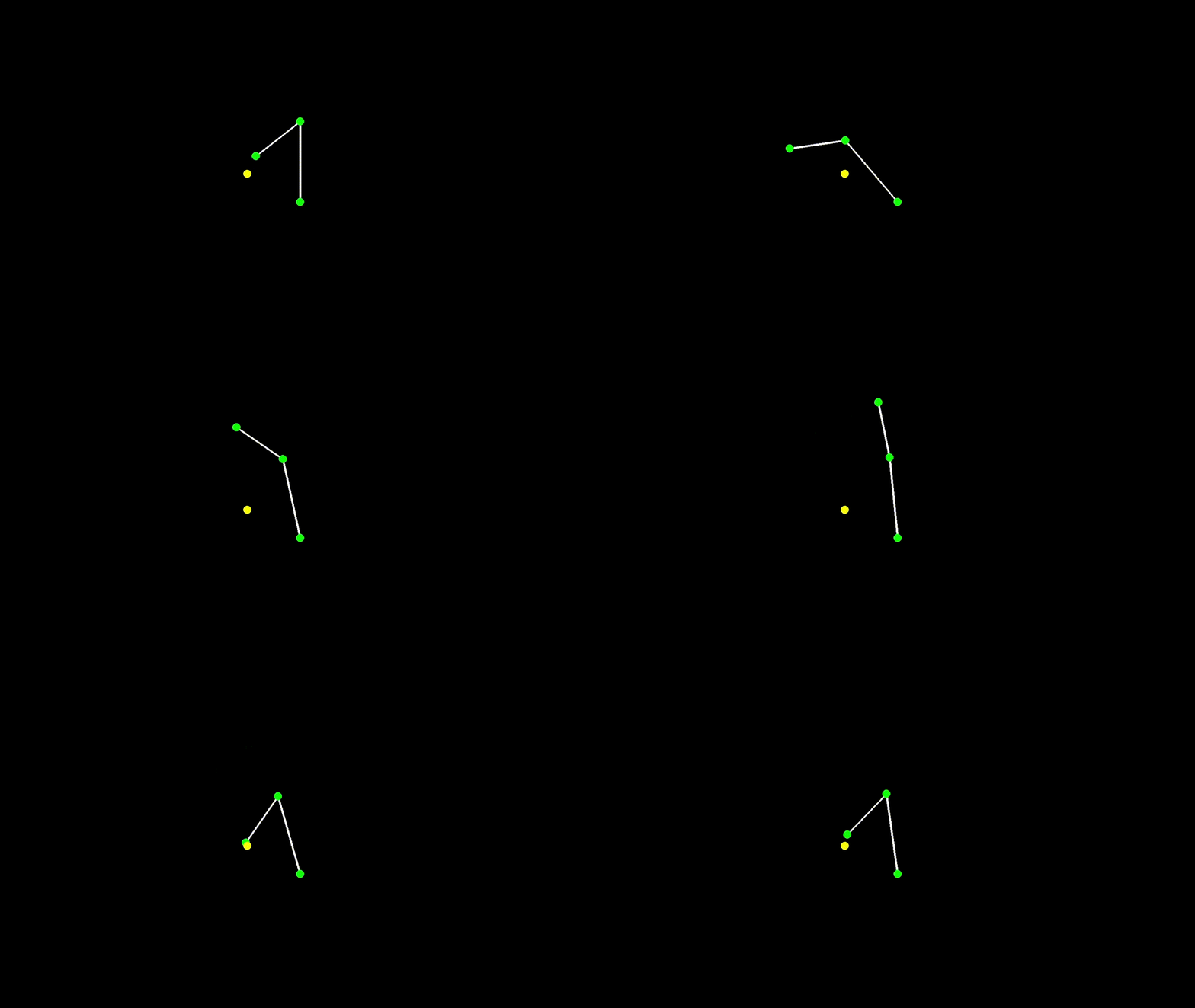
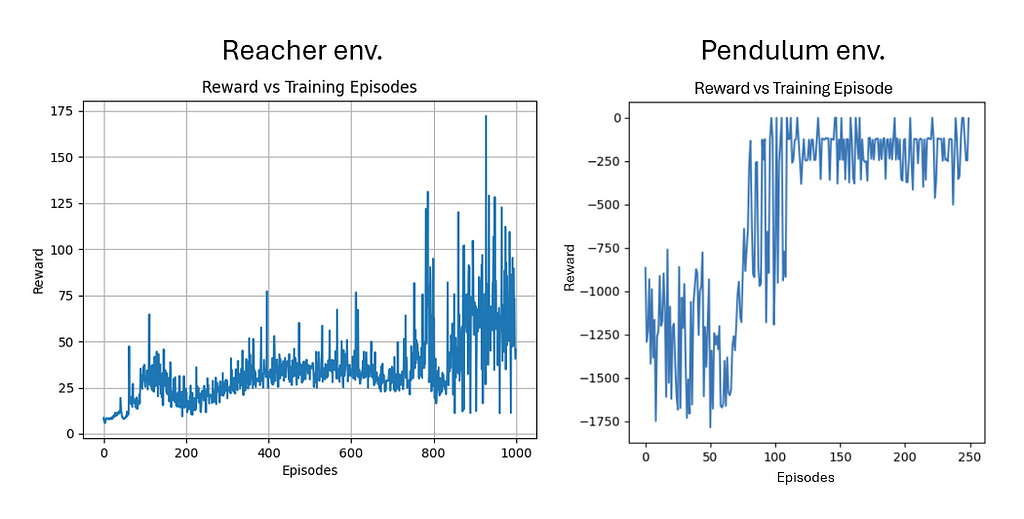
In training the SAC agent in both environments, I noticed that the action space of the problem affects the efficiency and the performance of the training. Indeed, when I trained the agent on the simple pendulum environment, the learning converged much faster and with lower oscillations. However, as the Reacher environment includes a more complicated continuous space of actions, the algorithm trained relatively well, but the big jump in the rewards was not seen as clearly. The Reacher was also trained on 4 times the number of episodes as that of the pendulum.

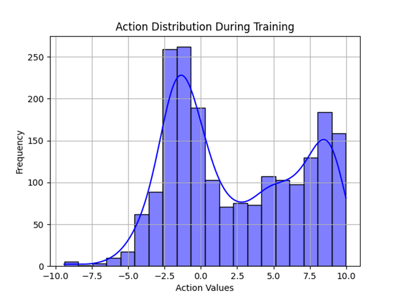
The action distribution below shows that the policy has a diverse range of actions that it explores through the training process until it converges on one optimal policy. The hallmark of entropy-regularised algorithms such as SAC comes from the increase in exploration. We can also notice that the peaks correspond to action values with high expected rewards which drives the policy to converge toward a more deterministic behaviour.

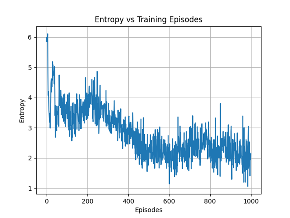
Speaking of a more deterministic behaviour, we observe that the entropy has decreased on average over the number of training episodes. However, this behaviour is expected, since the sole reason we want to maximise the entropy is to encourage more exploration. A higher exploration is mainly done early in the training process to exhaust most possible state-actions pairs that have higher returns.

Conclusion

The SAC algorithm is an off-policy RL framework that adopts a balance of exploitation and exploration through a new entropy term. The main objective function of the SAC algorithm includes maximising both the expected returns and the entropy during the training process, which address many of the issues the legacy frameworks suffer from. The use of twin Q-networks and automatic temperature tuning address high sample complexity, brittle convergence properties and complex hyperparameter tuning. SAC has proven to be highly effective in continuous control task domains. The results on action distribution and entropy reveal that the algorithm favours exploration in early training phases and diverse action sampling. As the agent trains, it converges to a more specific policy which reduces the entropy and reaches optimal actions. Consequently, it has been effectively used as an alternative for a wide range of domains in bioengineering for robotic control, drug discovery and drug delivery. Future implementations should focus on scaling the framework to more complex tasks and reducing its computational complexity.

References

Lillicrap, T.P., Hunt, J.J., Pritzel, A., Heess, N., Erez, T., Tassa, Y., Silver, D. and Wierstra, D. (2015). Continuous control with deep reinforcement learning. [online] arXiv.org. Available at: https://arxiv.org/abs/1509.02971.

Schulman, J., Wolski, F., Dhariwal, P., Radford, A. and Klimov, O. (2017). Proximal Policy Optimization Algorithms. [online] arXiv.org. Available at: https://arxiv.org/abs/1707.06347.

Haarnoja, T., Zhou, A., Abbeel, P. and Levine, S. (2018). Soft Actor-Critic: Off-Policy Maximum Entropy Deep Reinforcement Learning with a Stochastic Actor. arXiv:1801.01290 [cs, stat]. [online] Available at: https://arxiv.org/abs/1801.01290.

Du, H., Li, Z., Niyato, D., Yu, R., Xiong, Z., Xuemin, Shen and Dong In Kim (2023). Enabling AI-Generated Content (AIGC) Services in Wireless Edge Networks. doi:https://doi.org/10.48550/arxiv.2301.03220.

Svensson, H.G., Tyrchan, C., Engkvist, O. and Morteza Haghir Chehreghani (2024). Utilizing reinforcement learning for de novo drug design. Machine Learning, 113(7), pp.4811–4843. doi:https://doi.org/10.1007/s10994-024-06519-w.

quantumiracle (2019). GitHub — quantumiracle/Popular-RL-Algorithms: PyTorch implementation of Soft Actor-Critic (SAC), Twin Delayed DDPG (TD3), Actor-Critic (AC/A2C), Proximal Policy Optimization (PPO), QT-Opt, PointNet.. [online] GitHub. Available at: https://github.com/quantumiracle/Popular-RL-Algorithms [Accessed 12 Dec. 2024].

MrSyee (2019). GitHub — MrSyee/pg-is-all-you-need: Policy Gradient is all you need! A step-by-step tutorial for well-known PG methods. [online] GitHub. Available at: https://github.com/MrSyee/pg-is-all-you-need?tab=readme-ov-file.

---

Navigating Soft Actor-Critic Reinforcement Learning was originally published in Towards Data Science on Medium, where people are continuing the conversation by highlighting and responding to this story.

​Understanding the theory and implementation of SAC RL in the context of BioengineeringImage generated by the author using ChatGPT-4oIntroductionThe research domain of Reinforcement Learning (RL) has evolved greatly over the past years. The use of deep reinforcement learning methods such as Proximal Policy Optimisation (PPO) (Schulman, 2017) and Deep Deterministic Policy Gradient (DDPG) (Lillicrap, 2015) have enabled agents to solve tasks in high-dimensional environments. However, many of these model-free RL algorithms have struggled with stability during the training process. These challenges arise due to the brittle convergence properties, high variance in gradient estimation, very high sample complexity, and the sensitivity to hyperparameters in continuous action spaces. Given these problems, it is imperative to consider a newly devised RL algorithm that avoids such issues and expands applicability to complex, real-world problems. This new algorithm is the Soft Actor-Critic (SAC) deep RL network. (Haarnoja, 2018)Model Architecture of Soft Actor-Critic Networks. Image taken from (Du, 2023)SAC is an off-policy Actor-Critic deep RL algorithm which is designed to address the stability and efficiency constraints of its predecessors. The SAC algorithm is based on the maximum entropy RL framework which aims for the actor part of the network to maximise the expected reward, while maximising entropy. It combines off-policy updates with a more stable formulation of the stochastic Actor-Critic method. An off-policy algorithm enables faster learning and better sample efficiency using experience replay, unlike on-policy methods such as PPO, which require new samples for each gradient step. For on-policy methods such as PPO, for each gradient step in the learning process, new samples must be collected. The aim of using stochastic policies and maximising entropy comes to promote the robustness and exploration of the algorithm by encouraging more randomness in the actions. Additionally, unlike PPO and DDPG, SAC uses twin Q-networks with a separate Actor network and entropy tuning to improve the stability and convergence when combining off-policy learning with high dimensional, nonlinear function approximation.Off-policy RL methods have had a wide impact on bioengineering systems that improve patient lives. More specifically, RL has been applied to domains such as robotic arm control, drug delivery methods and most notably de novo drug design. (Svensson, 2024) Svensson et al. has used a number of on- and off-policy frameworks and different variants of replay buffers to learn a RNN-based molecule generation policy, to be active against DRD2 (a dopamine receptor). The paper realises that using experience replay across the board for high, intermediate and low scoring molecules has shown effects in improving the structural diversity and the number of active molecules generated. Replay buffers improve sample efficiency in training agents. They also reported that the use of off-policy methods and more specifically SAC, helps in promoting structural diversity by preventing mode collapse.Theoretical ExplanationSAC uses ‘soft’ value functions by introducing the objective function with an entropy term, Η(π(a|s)). Accordingly, the network seeks to maximise both the expected return of lifetime rewards and the entropy of the policy. The entropy of the policy is defined as the unpredictability of a random variable, which increases with the range of possible values. Thus, the new entropy regularised objective becomes:Entropy Regularised Objectiveα is the temperature parameter that balances between exploration and exploitation.In the implementation of soft value functions, we aim to maximise the entropy as the algorithm would assign equal probabilities to actions that have a similar Q-value. Maximising entropy also helps with preventing the agent from choosing actions that exploit inconsistencies in approximated Q-values. We can finally understand how SAC improves brittleness by allowing the network to explore more and not assign very high probabilities to one range of actions. This part is inspired by Vaishak V.Kumar’s explanation of the entropy maximisation in “Soft Actor-Critic Demystified”.The SAC paper authors discuss that since the state value function approximates the soft value, there is really no essential need to train separate function approximators for the policy, since they relate to the state value according to the following equation. However, training three separate approximators provided better convergence.Soft State Value FunctionThe three function approximator networks are characterised as follows:Policy Network (Actor): the stochastic policy outputs a set of actions sampled from a Gaussian distribution. The policy parameters are learned by minimising the Kullback-Leibler Divergence as provided in this equation:Minimising KL-DivergenceThe KL-divergence compares the relative entropy or the difference between two probability distributions. So, in the equation, we are trying to minimise the difference between the distributions of the policy function and the exponentiated Q-function normalised by a function Z. Since the target density function is the Q-function, which is differentiable, we apply a reparametrisation trick on the policy to reduce the estimation of the variance.Reparametrised Policyϵₜ is a vector sampled from a Gaussian distribution which describes the noise.The policy objective is then updated to the following expression:Policy ObjectiveThe policy objective is optimised using the following gradient estimation:Policy Gradient EstimatorQ-Network (Critic): includes two Q-value networks to estimate the expected reward for the state-action pairs. We minimise the soft Q-function parameters by using the soft Bellman residual provided here:Soft Q-function Objectivewhere:Immediate Q-valueThe soft Q-function objective minimises the square differences between the networks Q-value estimation and the immediate Q-value. The immediate Q-value (Q hat) is obtained from the reward of the current state-action pair added to the discounted expectation of the target value function in the following time stamp. Finally, the objective is optimised using a stochastic gradient estimation given by the following:Stochastic Gradient EstimatorTarget Value Network (Critic): a separate soft value function which helps in stabilising the training process. The soft value function approximator minimises the squared residual error as follows:Soft Value Function ObjectiveThis soft value function objective minimises the square differences between the value function and the expectation of the Q-value plus the entropy of the policy function π. The negative log part of this objective describes the entropy of the policy function. We also know that the information entropy is calculated using a negative sign to output a positive entropy value, since the log of a probability value (between 0 and 1) will be negative. Similarly, the objective is optimised using an unbiased gradient estimator, given in the following expression:Unbiased Gradient EstimatorCode ImplementationThe code implemented in this article is taken from the following Github repository (quantumiracle, 2023):GitHub – quantumiracle/Popular-RL-Algorithms: PyTorch implementation of Soft Actor-Critic (SAC), Twin Delayed DDPG (TD3), Actor-Critic (AC/A2C), Proximal Policy Optimization (PPO), QT-Opt, PointNet..pip install gymnasium torchSAC relies on environments that use continuous action spaces, so the simulation provided uses the robotic arm ‘Reacher’ environment for the most part and the Pendulum-v1 environment in the gymnasium package.The Pendulum environment was run on a different repository that implements the same algorithm but with less deprecated libraries given by (MrSyee, 2020):GitHub – MrSyee/pg-is-all-you-need: Policy Gradient is all you need! A step-by-step tutorial for well-known PG methods.In terms of the network architectures, as mentioned in the Theory Explanation, there are three main components:Policy Network: implements a Gaussian Actor network computing the mean and log standard deviation for the action distribution.class PolicyNetwork(nn.Module): def __init__(self, state_dim, action_dim, hidden_dim): super(PolicyNetwork, self).__init__() self.fc1 = nn.Linear(state_dim, hidden_dim) self.fc2 = nn.Linear(hidden_dim, hidden_dim) self.mean = nn.Linear(hidden_dim, action_dim) self.log_std = nn.Linear(hidden_dim, action_dim) def forward(self, state): x = F.relu(self.fc1(state)) x = F.relu(self.fc2(x)) mean = self.mean(x) log_std = torch.clamp(self.log_std(x), -20, 2) # Limit log_std to prevent instability return mean, log_stdSoft Q-Network: estimates the expected future reward given from a state-action pair for a defined optimal policy.class SoftQNetwork(nn.Module): def __init__(self, state_dim, action_dim, hidden_dim): super(SoftQNetwork, self).__init__() self.fc1 = nn.Linear(state_dim + action_dim, hidden_dim) self.fc2 = nn.Linear(hidden_dim, hidden_dim) self.out = nn.Linear(hidden_dim, 1) def forward(self, state, action): x = torch.cat([state, action], dim=-1) x = F.relu(self.fc1(x)) x = F.relu(self.fc2(x)) return self.out(x)Value Network: estimates the state value.class ValueNetwork(nn.Module): def __init__(self, state_dim, hidden_dim): super(ValueNetwork, self).__init__() self.fc1 = nn.Linear(state_dim, hidden_dim) self.fc2 = nn.Linear(hidden_dim, hidden_dim) self.out = nn.Linear(hidden_dim, 1) def forward(self, state): x = F.relu(self.fc1(state)) x = F.relu(self.fc2(x)) return self.out(x)The following snippet offers the key steps in updating the different variables corresponding to the SAC algorithm. As it starts by sampling a batch from the replay buffer for experience replay. Then, before computing the gradients, they are initialised to zero to ensure that gradients from previous batches are not accumulated. Then performs backpropagation and updates the weights of the network during training. The target and loss values are then updated for the Q-networks. These steps take place for all three methods.def update(batch_size, reward_scale, gamma=0.99, soft_tau=1e-2): # Sample a batch state, action, reward, next_state, done = replay_buffer.sample(batch_size) state, next_state, action, reward, done = map(lambda x: torch.FloatTensor(x).to(device), [state, next_state, action, reward, done]) # Update Q-networks target_value = target_value_net(next_state) target_q = reward + (1 – done) * gamma * target_value q1_loss = F.mse_loss(soft_q_net1(state, action), target_q.detach()) q2_loss = F.mse_loss(soft_q_net2(state, action), target_q.detach()) soft_q_optimizer1.zero_grad() q1_loss.backward() soft_q_optimizer1.step() soft_q_optimizer2.zero_grad() q2_loss.backward() soft_q_optimizer2.step() # Update Value Network predicted_q = torch.min(soft_q_net1(state, action), soft_q_net2(state, action)) value_loss = F.mse_loss(value_net(state), predicted_q – alpha * log_prob) value_optimizer.zero_grad() value_loss.backward() value_optimizer.step() # Update Policy Network new_action, log_prob, _, _, _ = policy_net.evaluate(state) policy_loss = (alpha * log_prob – predicted_q).mean() policy_optimizer.zero_grad() policy_loss.backward() policy_optimizer.step() # Soft Update Target Network for target_param, param in zip(target_value_net.parameters(), value_net.parameters()): target_param.data.copy_(soft_tau * param.data + (1 – soft_tau) * target_param.data)Finally, to run the code in the sac.py file, just run the following commands:python sac.py –trainpython sac.py –testResults and VisualisationTraining a ‘Reacher’ Robotic Arm, (generated by the author)In training the SAC agent in both environments, I noticed that the action space of the problem affects the efficiency and the performance of the training. Indeed, when I trained the agent on the simple pendulum environment, the learning converged much faster and with lower oscillations. However, as the Reacher environment includes a more complicated continuous space of actions, the algorithm trained relatively well, but the big jump in the rewards was not seen as clearly. The Reacher was also trained on 4 times the number of episodes as that of the pendulum.Learning Performance by Maximising Reward (generated by the author)The action distribution below shows that the policy has a diverse range of actions that it explores through the training process until it converges on one optimal policy. The hallmark of entropy-regularised algorithms such as SAC comes from the increase in exploration. We can also notice that the peaks correspond to action values with high expected rewards which drives the policy to converge toward a more deterministic behaviour.Action Space Usage Distribution (generated by the author)Speaking of a more deterministic behaviour, we observe that the entropy has decreased on average over the number of training episodes. However, this behaviour is expected, since the sole reason we want to maximise the entropy is to encourage more exploration. A higher exploration is mainly done early in the training process to exhaust most possible state-actions pairs that have higher returns.Entropy Valuation Over Training Episodes (generated by the author)ConclusionThe SAC algorithm is an off-policy RL framework that adopts a balance of exploitation and exploration through a new entropy term. The main objective function of the SAC algorithm includes maximising both the expected returns and the entropy during the training process, which address many of the issues the legacy frameworks suffer from. The use of twin Q-networks and automatic temperature tuning address high sample complexity, brittle convergence properties and complex hyperparameter tuning. SAC has proven to be highly effective in continuous control task domains. The results on action distribution and entropy reveal that the algorithm favours exploration in early training phases and diverse action sampling. As the agent trains, it converges to a more specific policy which reduces the entropy and reaches optimal actions. Consequently, it has been effectively used as an alternative for a wide range of domains in bioengineering for robotic control, drug discovery and drug delivery. Future implementations should focus on scaling the framework to more complex tasks and reducing its computational complexity.ReferencesLillicrap, T.P., Hunt, J.J., Pritzel, A., Heess, N., Erez, T., Tassa, Y., Silver, D. and Wierstra, D. (2015). Continuous control with deep reinforcement learning. [online] arXiv.org. Available at: https://arxiv.org/abs/1509.02971.Schulman, J., Wolski, F., Dhariwal, P., Radford, A. and Klimov, O. (2017). Proximal Policy Optimization Algorithms. [online] arXiv.org. Available at: https://arxiv.org/abs/1707.06347.Haarnoja, T., Zhou, A., Abbeel, P. and Levine, S. (2018). Soft Actor-Critic: Off-Policy Maximum Entropy Deep Reinforcement Learning with a Stochastic Actor. arXiv:1801.01290 [cs, stat]. [online] Available at: https://arxiv.org/abs/1801.01290.Du, H., Li, Z., Niyato, D., Yu, R., Xiong, Z., Xuemin, Shen and Dong In Kim (2023). Enabling AI-Generated Content (AIGC) Services in Wireless Edge Networks. doi:https://doi.org/10.48550/arxiv.2301.03220.Svensson, H.G., Tyrchan, C., Engkvist, O. and Morteza Haghir Chehreghani (2024). Utilizing reinforcement learning for de novo drug design. Machine Learning, 113(7), pp.4811–4843. doi:https://doi.org/10.1007/s10994-024-06519-w.quantumiracle (2019). GitHub — quantumiracle/Popular-RL-Algorithms: PyTorch implementation of Soft Actor-Critic (SAC), Twin Delayed DDPG (TD3), Actor-Critic (AC/A2C), Proximal Policy Optimization (PPO), QT-Opt, PointNet.. [online] GitHub. Available at: https://github.com/quantumiracle/Popular-RL-Algorithms [Accessed 12 Dec. 2024].MrSyee (2019). GitHub — MrSyee/pg-is-all-you-need: Policy Gradient is all you need! A step-by-step tutorial for well-known PG methods. [online] GitHub. Available at: https://github.com/MrSyee/pg-is-all-you-need?tab=readme-ov-file.Navigating Soft Actor-Critic Reinforcement Learning was originally published in Towards Data Science on Medium, where people are continuing the conversation by highlighting and responding to this story.  soft-actor-critic, optimisation, machine-learning, reinforcement-learning, bioengineering Towards Data Science – MediumRead More

Add to favorites