Understanding the Unbiased Estimation of Population Variance

In statistics, a common point of confusion for many learners is why we divide by n−1 when calculating sample variance, rather than simply using n, the number of observations in the sample. This choice may seem small but is a critical adjustment that corrects for a natural bias that occurs when we estimate the variance of a population from a sample. Let’s walk through the reasoning in simple language, with examples to understand why dividing by n−1, known as Bessel’s correction, is necessary.

The core concept of correction (in Bessel’s correction), is that we tend to correct our estimation, but a clear question is estimation of what? So by applying Bessel’s correction we tend to correct the estimation of deviations calculated from our assumed sample mean, our assumed sample mean will rarely ever co-inside with the actual population mean, so it’s safe to assume that in 99.99% (even more than that in real) cases our sample mean would not be equal to the population mean. We do all the calculations based on this assumed sample mean, that is we estimate the population parameters through the mean of this sample.

Reading further down the blog, one would get a clear intuition that why in all of those 99.99% cases (in all the cases except leaving the one, in which sample mean = population mean), we tend to underestimate the deviations from actual deviations, so to compensate this underestimation error, diving by a smaller number than ’n’ do the job, so diving by n-1 instead of n, accounts for the compensation of the underestimation that is done in calculating the deviations from the sample mean.

Start reading down from here and you’ll eventually understand…

Sample Variance vs. Population Variance

When we have an entire population of data points, the variance is calculated by finding the mean (average), then determining how each point deviates from this mean, squaring these deviations, summing them up, and finally dividing by n, the total number of points in the population. This gives us the population variance.

However, if we don’t have data for an entire population and are instead working with just a sample, we estimate the population variance. But here lies the problem: when using only a sample, we don’t know the true population mean (denoted as μ), so we use the sample mean (x_bar) instead.

The Problem of Underestimation

To understand why we divide by n−1 in the case of samples, we need to look closely at what happens when we use the sample mean rather than the population mean. For real-life applications, relying on sample statistics is the only option we have. Here’s how it works:

When we calculate variance in a sample, we find each data point’s deviation from the sample mean, square those deviations, and then take the average of these squared deviations. However, the sample mean is usually not exactly equal to the population mean. Due to this difference, using the sample mean tends to underestimate the true spread or variance in the population.

Let’s break it down with all possible cases that can happen (three different cases), I’ll give a detailed walkthrough on the first case, same principle applies to the other two cases as well, detailed walkthrough has been given for case 1.

1. When the Sample Mean is Less Than the Population Mean (x_bar < population mean)

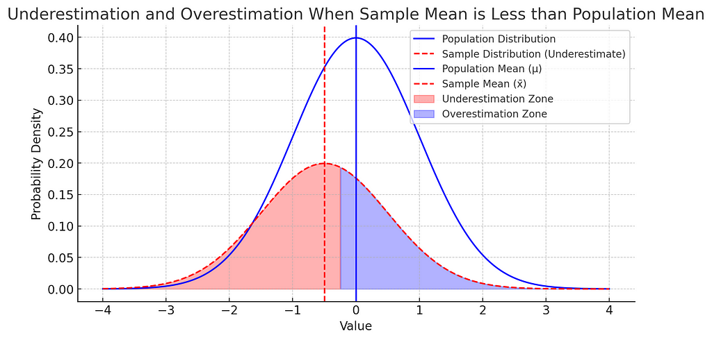
If our sample mean (x_bar) is less than the population mean (μ), then many of the points in the sample will be closer to (x_bar) than they would be to μ. As a result, the distances (deviations) from the mean are smaller on average, leading to a smaller variance calculation. This means we’re underestimating the actual variance.

Explanation of the graph given below — The smaller normal distribution is of our sample and the bigger normal distribution is of our population (in the above case where x_bar < population mean), the plot would look like the one shown below.

As we have data points of our sample, because that’s what we can collect, can’t collect all the data points of the population because that’s simply not possible. For all the data points in our sample in this case, from negative infinity, to the mid point of x_bar and population mean, the absolute or squared difference (deviations) between the sample points and population mean would be greater than the absolute or squared difference (deviations) between sample points and sample mean and on the right side of the midpoint till positive infinity, the deviations calculated with respect to sample mean would be greater than the deviations calculated using population mean. The region is indicated in the graph below for the above case, due to the symmetric nature of the normal curve we can surely say that the underestimation zone would be larger than the overestimation zone which is also highlighted in the graph below, which results in an overall underestimation of the deviations.

So to compensate the underestimation, we divide the deviations by a number smaller than sample size ’n’, which is ‘n-1’ which is known as Bessel’s correction.

2. When the Sample Mean is Greater Than the Population Mean

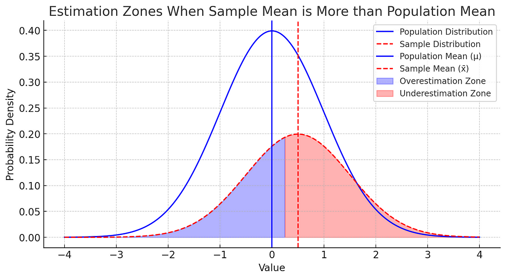
If the sample mean is greater than the population mean, we have the reverse situation: data points on the low end of the sample will be closer to x_bar than to μ, still resulting in an underestimation of variance.

Based on the details laid above, it’s clear that in this case also underestimation zone is larger than the overestimation zone, so in this case also we will account for this underestimation by dividing the deviations by ‘n-1’ instead of n.

3. When the Sample Mean is Exactly Equal to the Population Mean (0.000001%)

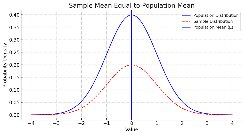
This case is rare, and only if the sample mean is perfectly aligned with the population mean would our estimate be unbiased. However, this alignment almost never happens by chance, so we generally assume that we’re underestimating.

Clearly, deviations calculated for the sample points with respect to sample mean are exactly the same as the deviations calculated with respect to the population mean, because the sample mean and population mean both are equal. This would yield no underestimation or overestimation zone.

In short, any difference between x_bar and μ (which almost always occurs) leads us to underestimate the variance. This is why we need to make a correction by dividing by n−1, which accounts for this bias.

Why Dividing by n−1 Corrects This Bias: Bessel’s Correction

Dividing by n−1 is called Bessel’s correction and compensates for the natural underestimation bias in sample variance. When we divide by n−1, we’re effectively making a small adjustment that spreads out our variance estimate, making it a better reflection of the true population variance.

One can relate all this to degrees of freedom too , some knowledge of dofs are required to understand from the viewpoint of degrees of freedom-

In a sample, one degree of freedom is “used up” by calculating the sample mean. This leaves us with n−1 independent data points that contribute information about the variance, which is why we divide by n−1 rather than n.

Why Does This Adjustment Matter More with Small Samples?

If our sample size is very small, the difference between dividing by n and n−1 becomes more significant. For instance, if you have a sample size of 10:

• Dividing by n would mean dividing by 10, which may greatly underestimate the variance.
• Dividing by n−1 or 9, provides a better estimate, compensating for the small sample.

But if your sample size is large (say, 10,000), the difference between dividing by 10,000 or 9,999 is tiny, so the impact of Bessel’s correction is minimal.

Consequences of Not Using Bessel’s Correction

If we don’t use Bessel’s correction, our sample variance will generally underestimate the population variance. This can have cascading effects, especially in statistical modelling and hypothesis testing, where accurate variance estimates are crucial for drawing reliable conclusions.

For instance:

• Confidence intervals: Variance estimates influence the width of confidence intervals around a sample mean. Underestimating variance could lead to narrower intervals, giving a false impression of precision.
• Hypothesis tests: Many statistical tests, such as the t-test, rely on accurate variance estimates to determine if observed effects are significant. Underestimating variance could make it harder to detect true differences.

Why Not Divide by n−2 or n−3?

The choice to divide by n−1 isn’t arbitrary. While we won’t go into the detailed proof here, it’s grounded in mathematical theory. Dividing by n−1 provides an unbiased estimate of the population variance when calculated from a sample. Other adjustments, such as n−2, would overcorrect and lead to an overestimation of variance.

A Practical Example to Illustrate Bessel’s Correction

Imagine you have a small population with a mean weight of 70 kg. Now let’s say you take a sample of 5 people from this population, and their weights (in kg) are 68, 69, 70, 71, and 72. The sample mean is exactly 70 kg — identical to the population mean by coincidence.

Now suppose we calculate the variance:

1. Without Bessel’s correction: we’d divide the sum of squared deviations by n=5.
2. With Bessel’s correction: we divide by n−1=4.

Using Bessel’s correction in this way slightly increases our estimate of the variance, making it closer to what the population variance would be if we calculated it from the whole population instead of just a sample.

Conclusion

Dividing by n−1 when calculating sample variance may seem like a small change, but it’s essential to achieve an unbiased estimate of the population variance. This adjustment, known as Bessel’s correction, accounts for the underestimation that occurs due to relying on the sample mean instead of the true population mean.

In summary:

• Using n−1 compensates for the fact that we’re basing variance on a sample mean, which tends to underestimate true variability.
• The correction is especially important with small sample sizes, where dividing by n would significantly distort the variance estimate.
• This practice is fundamental in statistics, affecting everything from confidence intervals to hypothesis tests, and is a cornerstone of reliable data analysis.

By understanding and applying Bessel’s correction, we ensure that our statistical analyses reflect the true nature of the data we study, leading to more accurate and trustworthy conclusions.

---

Bessel’s Correction: Why Do We Divide by n−1 Instead of n in Sample Variance? was originally published in Towards Data Science on Medium, where people are continuing the conversation by highlighting and responding to this story.

​Understanding the Unbiased Estimation of Population VarianceIn statistics, a common point of confusion for many learners is why we divide by n−1 when calculating sample variance, rather than simply using n, the number of observations in the sample. This choice may seem small but is a critical adjustment that corrects for a natural bias that occurs when we estimate the variance of a population from a sample. Let’s walk through the reasoning in simple language, with examples to understand why dividing by n−1, known as Bessel’s correction, is necessary.The core concept of correction (in Bessel’s correction), is that we tend to correct our estimation, but a clear question is estimation of what? So by applying Bessel’s correction we tend to correct the estimation of deviations calculated from our assumed sample mean, our assumed sample mean will rarely ever co-inside with the actual population mean, so it’s safe to assume that in 99.99% (even more than that in real) cases our sample mean would not be equal to the population mean. We do all the calculations based on this assumed sample mean, that is we estimate the population parameters through the mean of this sample.Reading further down the blog, one would get a clear intuition that why in all of those 99.99% cases (in all the cases except leaving the one, in which sample mean = population mean), we tend to underestimate the deviations from actual deviations, so to compensate this underestimation error, diving by a smaller number than ’n’ do the job, so diving by n-1 instead of n, accounts for the compensation of the underestimation that is done in calculating the deviations from the sample mean.Start reading down from here and you’ll eventually understand…Sample Variance vs. Population VarianceWhen we have an entire population of data points, the variance is calculated by finding the mean (average), then determining how each point deviates from this mean, squaring these deviations, summing them up, and finally dividing by n, the total number of points in the population. This gives us the population variance.However, if we don’t have data for an entire population and are instead working with just a sample, we estimate the population variance. But here lies the problem: when using only a sample, we don’t know the true population mean (denoted as μ), so we use the sample mean (x_bar) instead.The Problem of UnderestimationTo understand why we divide by n−1 in the case of samples, we need to look closely at what happens when we use the sample mean rather than the population mean. For real-life applications, relying on sample statistics is the only option we have. Here’s how it works:When we calculate variance in a sample, we find each data point’s deviation from the sample mean, square those deviations, and then take the average of these squared deviations. However, the sample mean is usually not exactly equal to the population mean. Due to this difference, using the sample mean tends to underestimate the true spread or variance in the population.Let’s break it down with all possible cases that can happen (three different cases), I’ll give a detailed walkthrough on the first case, same principle applies to the other two cases as well, detailed walkthrough has been given for case 1.1. When the Sample Mean is Less Than the Population Mean (x_bar < population mean)If our sample mean (x_bar) is less than the population mean (μ), then many of the points in the sample will be closer to (x_bar) than they would be to μ. As a result, the distances (deviations) from the mean are smaller on average, leading to a smaller variance calculation. This means we’re underestimating the actual variance.Explanation of the graph given below — The smaller normal distribution is of our sample and the bigger normal distribution is of our population (in the above case where x_bar < population mean), the plot would look like the one shown below.As we have data points of our sample, because that’s what we can collect, can’t collect all the data points of the population because that’s simply not possible. For all the data points in our sample in this case, from negative infinity, to the mid point of x_bar and population mean, the absolute or squared difference (deviations) between the sample points and population mean would be greater than the absolute or squared difference (deviations) between sample points and sample mean and on the right side of the midpoint till positive infinity, the deviations calculated with respect to sample mean would be greater than the deviations calculated using population mean. The region is indicated in the graph below for the above case, due to the symmetric nature of the normal curve we can surely say that the underestimation zone would be larger than the overestimation zone which is also highlighted in the graph below, which results in an overall underestimation of the deviations.So to compensate the underestimation, we divide the deviations by a number smaller than sample size ’n’, which is ‘n-1’ which is known as Bessel’s correction.Plot produced by python code using matplotlib library, Image Source (Author)2. When the Sample Mean is Greater Than the Population MeanIf the sample mean is greater than the population mean, we have the reverse situation: data points on the low end of the sample will be closer to x_bar than to μ, still resulting in an underestimation of variance.Based on the details laid above, it’s clear that in this case also underestimation zone is larger than the overestimation zone, so in this case also we will account for this underestimation by dividing the deviations by ‘n-1’ instead of n.Plot produced by python code using matplotlib library, Image Source (Author)3. When the Sample Mean is Exactly Equal to the Population Mean (0.000001%)This case is rare, and only if the sample mean is perfectly aligned with the population mean would our estimate be unbiased. However, this alignment almost never happens by chance, so we generally assume that we’re underestimating.Clearly, deviations calculated for the sample points with respect to sample mean are exactly the same as the deviations calculated with respect to the population mean, because the sample mean and population mean both are equal. This would yield no underestimation or overestimation zone.Plot produced by python code using matplotlib library, Image Source (Author)In short, any difference between x_bar and μ (which almost always occurs) leads us to underestimate the variance. This is why we need to make a correction by dividing by n−1, which accounts for this bias.Why Dividing by n−1 Corrects This Bias: Bessel’s CorrectionDividing by n−1 is called Bessel’s correction and compensates for the natural underestimation bias in sample variance. When we divide by n−1, we’re effectively making a small adjustment that spreads out our variance estimate, making it a better reflection of the true population variance.One can relate all this to degrees of freedom too , some knowledge of dofs are required to understand from the viewpoint of degrees of freedom-In a sample, one degree of freedom is “used up” by calculating the sample mean. This leaves us with n−1 independent data points that contribute information about the variance, which is why we divide by n−1 rather than n.Why Does This Adjustment Matter More with Small Samples?If our sample size is very small, the difference between dividing by n and n−1 becomes more significant. For instance, if you have a sample size of 10:Dividing by n would mean dividing by 10, which may greatly underestimate the variance.Dividing by n−1 or 9, provides a better estimate, compensating for the small sample.But if your sample size is large (say, 10,000), the difference between dividing by 10,000 or 9,999 is tiny, so the impact of Bessel’s correction is minimal.Consequences of Not Using Bessel’s CorrectionIf we don’t use Bessel’s correction, our sample variance will generally underestimate the population variance. This can have cascading effects, especially in statistical modelling and hypothesis testing, where accurate variance estimates are crucial for drawing reliable conclusions.For instance:Confidence intervals: Variance estimates influence the width of confidence intervals around a sample mean. Underestimating variance could lead to narrower intervals, giving a false impression of precision.Hypothesis tests: Many statistical tests, such as the t-test, rely on accurate variance estimates to determine if observed effects are significant. Underestimating variance could make it harder to detect true differences.Why Not Divide by n−2 or n−3?The choice to divide by n−1 isn’t arbitrary. While we won’t go into the detailed proof here, it’s grounded in mathematical theory. Dividing by n−1 provides an unbiased estimate of the population variance when calculated from a sample. Other adjustments, such as n−2, would overcorrect and lead to an overestimation of variance.A Practical Example to Illustrate Bessel’s CorrectionImagine you have a small population with a mean weight of 70 kg. Now let’s say you take a sample of 5 people from this population, and their weights (in kg) are 68, 69, 70, 71, and 72. The sample mean is exactly 70 kg — identical to the population mean by coincidence.Now suppose we calculate the variance:Without Bessel’s correction: we’d divide the sum of squared deviations by n=5.With Bessel’s correction: we divide by n−1=4.Using Bessel’s correction in this way slightly increases our estimate of the variance, making it closer to what the population variance would be if we calculated it from the whole population instead of just a sample.ConclusionDividing by n−1 when calculating sample variance may seem like a small change, but it’s essential to achieve an unbiased estimate of the population variance. This adjustment, known as Bessel’s correction, accounts for the underestimation that occurs due to relying on the sample mean instead of the true population mean.In summary:Using n−1 compensates for the fact that we’re basing variance on a sample mean, which tends to underestimate true variability.The correction is especially important with small sample sizes, where dividing by n would significantly distort the variance estimate.This practice is fundamental in statistics, affecting everything from confidence intervals to hypothesis tests, and is a cornerstone of reliable data analysis.By understanding and applying Bessel’s correction, we ensure that our statistical analyses reflect the true nature of the data we study, leading to more accurate and trustworthy conclusions.Bessel’s Correction: Why Do We Divide by n−1 Instead of n in Sample Variance? was originally published in Towards Data Science on Medium, where people are continuing the conversation by highlighting and responding to this story.  interview, machine-learning, mathematics, normal-distribution, statistics Towards Data Science – MediumRead More

Add to favorites