How to animate plots with OpenCV and Matplotlib

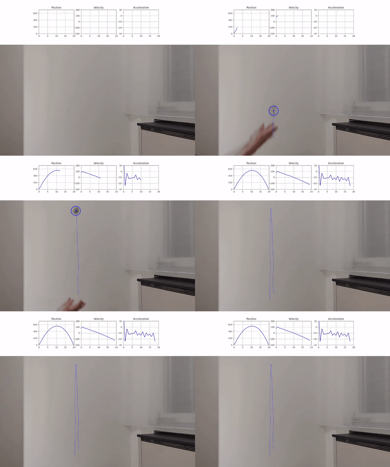
In Computer Vision a fundamental goal is to extract meaningful information from static images or video sequences. To understand these signals, it is often helpful to visualize them.

For example when tracking individual cars on a highway, we could draw bounding boxes around them or in the case of detecting problems in a product line on a conveyor belt, we could use a distinct color for anomalies. But what if the extracted information is of a more numerical nature and you want to visualize the time dynamics of this signal?

Just showing the value as a number on the screen might not give you enough insight, especially when the signal is changing rapidly. In these cases a great way to visualize the signal is a plot with a time axis. In this post I am going to show you how you can combine the power of OpenCV and Matplotlib to create animated real-time visualizations of such signals.

The code and video I used for this project is available on GitHub:

GitHub – trflorian/ball-tracking-live-plot: Tracking a ball using OpenCV and plotting the trajectory using Matplotlib

Plotting a Ball Trajectory

Let’s explore a toy problem where I recorded a video of a ball thrown vertically into the air. The goal is to track the ball in the video and plot it’s position p(t), velocity v(t) and acceleration a(t) over time.

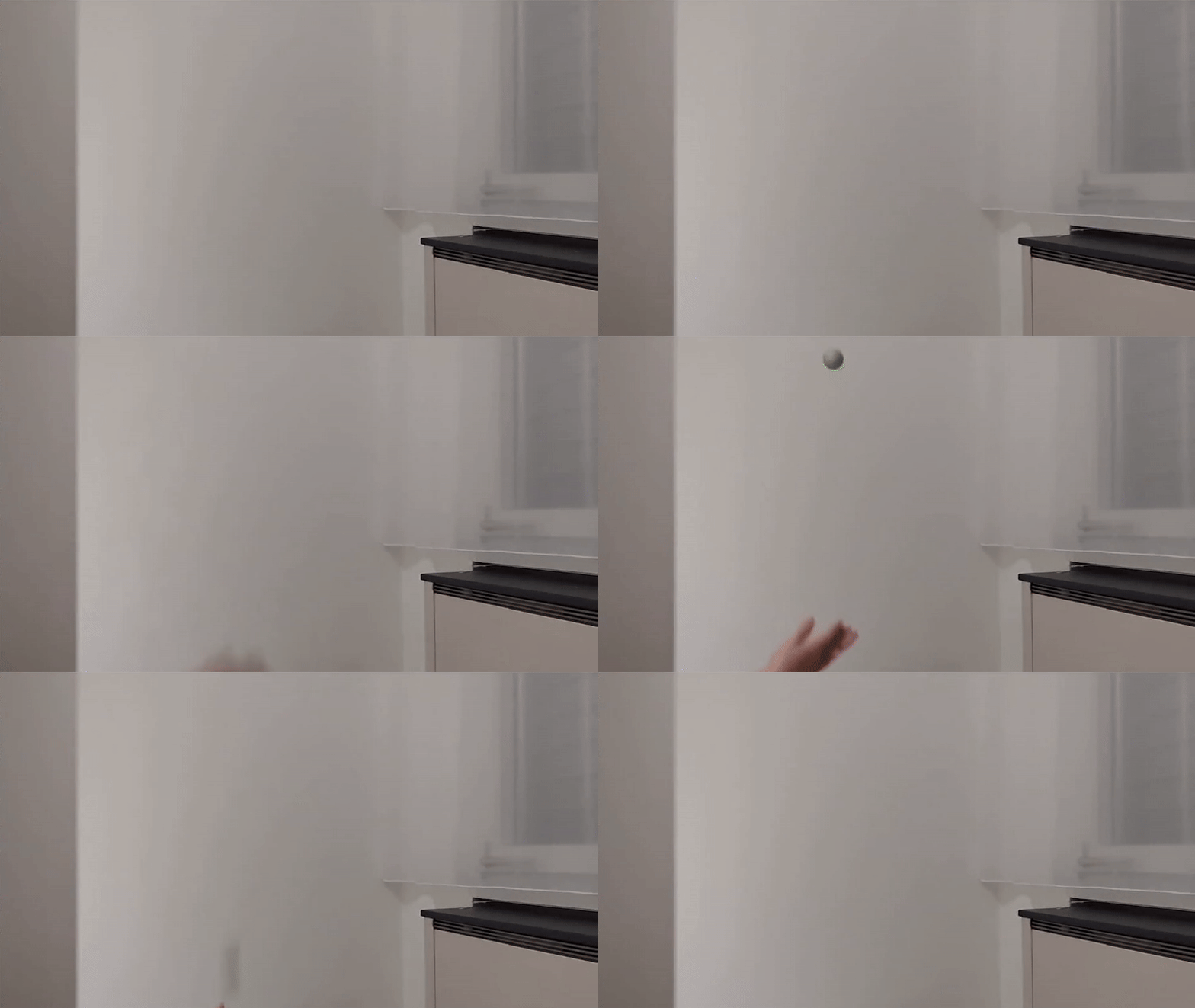
Let’s define our reference frame to be the camera and for simplicity we only track the vertical position of the ball in the image. We expect the position to be a parabola, the velocity to linearly decrease and the acceleration to be constant.

Ball Segmentation

In a first step we need to identify the ball in each frame of the video sequence. Since the camera remains static, an easy way to detect the ball is using a background subtraction model, combined with a color model to remove the hand in the frame.

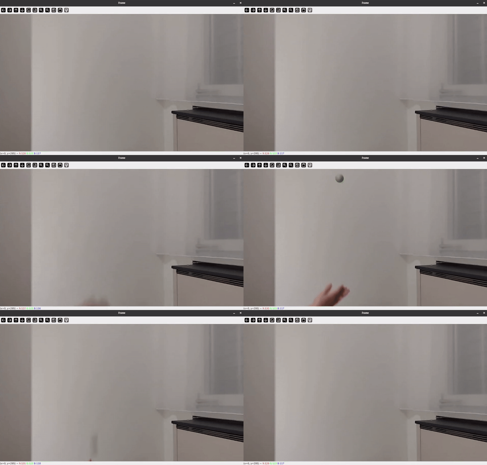
First let’s get our video clip displayed with a simple loop using VideoCapture from OpenCV. We simply restart the video clip once it has reached its end. We also make sure to playback the video at the original frame rate by calculating the sleep_time in milliseconds based on the FPS of the video. Also make sure to release the resources at the end and close the windows.

import cv2

cap = cv2.VideoCapture("ball.mp4")
fps = int(cap.get(cv2.CAP_PROP_FPS))

while True:
    ret, frame = cap.read()
    if not ret:
        cap.set(cv2.CAP_PROP_POS_FRAMES, 0)
        continue

    cv2.imshow("Frame", frame)

    sleep_time = 1000 // fps
    key = cv2.waitKey(sleep_time) & 0xFF
    if key & 0xFF == ord("q"):
        break

cap.release()
cv2.destroyAllWindows()

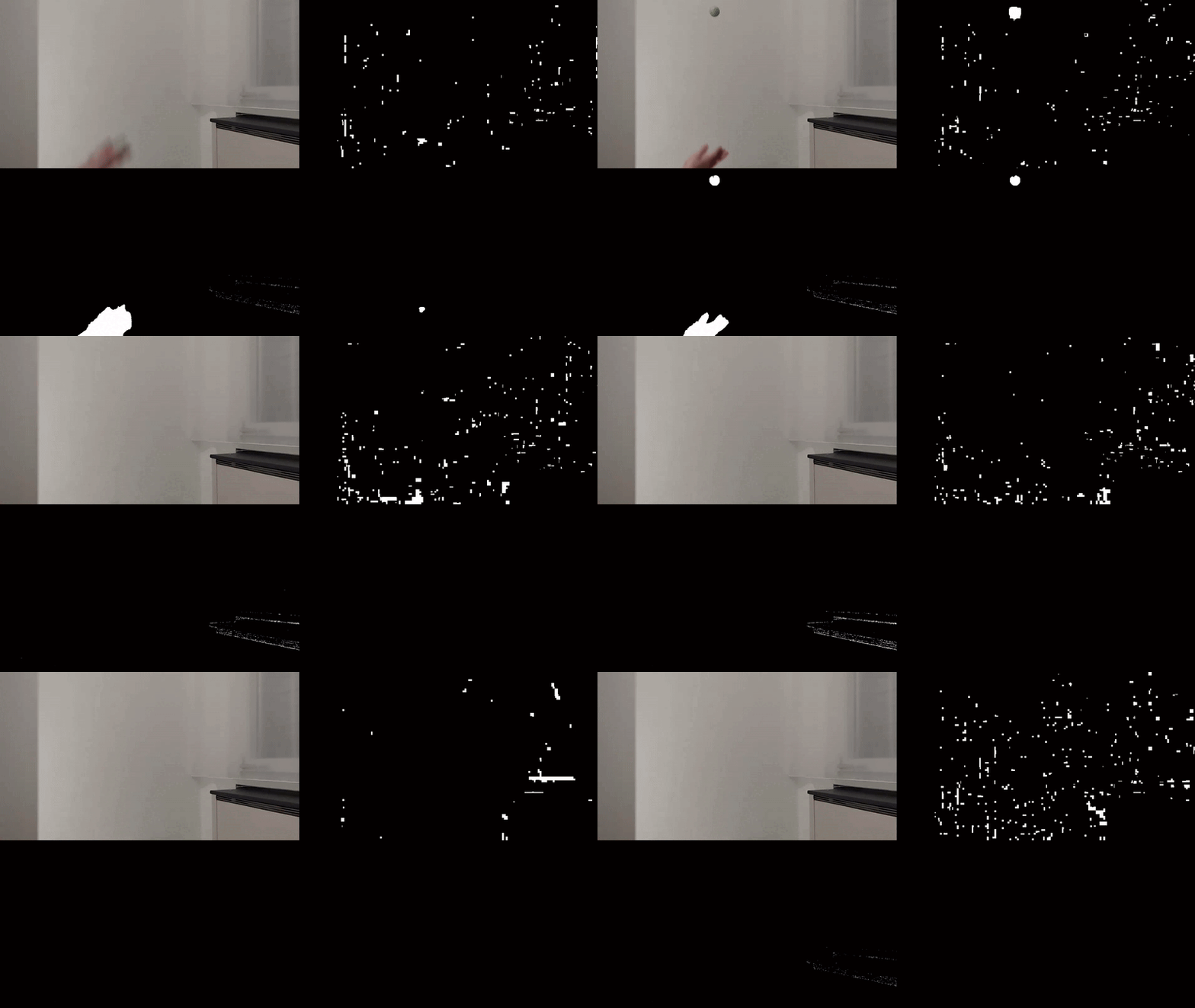
Let’s first work on extracting a binary segmentation mask for the ball. This essentially means that we want to create a mask that is active for pixels of the ball and inactive for all other pixels. To do this, I will combine two masks: a motion mask and a color mask. The motion mask extracts the moving parts and the color mask mainly gets rid of the hand in the frame.

For the color filter, we can convert the image to the HSV color space and select a specific hue range (20–100) that contains the green colors of the ball but no skin color tones. I don’t filter on the saturation or brightness values, so we can use the full range (0–255).

# filter based on color
hsv = cv2.cvtColor(frame, cv2.COLOR_BGR2HSV)
mask_color = cv2.inRange(hsv, (20, 0, 0), (100, 255, 255))

To create a motion mask we can use a simple background subtraction model. We use the first frame of the video for the background by setting the learning rate to 1. In the loop, we apply the background model to get the foreground mask, but don’t integrate new frames into it by setting the learning rate to 0.

...

# initialize background model
bg_sub = cv2.createBackgroundSubtractorMOG2(varThreshold=50, detectShadows=False)
ret, frame0 = cap.read()
if not ret:
    print("Error: cannot read video file")
    exit(1)
bg_sub.apply(frame0, learningRate=1.0)

while True:
  ...
  # filter based on motion
  mask_fg = bg_sub.apply(frame, learningRate=0)

In the next step, we can combine the two masks and apply a opening morphology to get rid of the small noise and we end up with a perfect segmentation of the ball.

# combine both masks
mask = cv2.bitwise_and(mask_color, mask_fg)
mask = cv2.morphologyEx(
    mask, cv2.MORPH_OPEN, cv2.getStructuringElement(cv2.MORPH_ELLIPSE, (13, 13))
)

Tracking the Ball

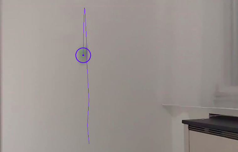
The only thing we’re left with is our ball in the mask. To track the center of the ball, I first extract the contour of the ball and then take the center of its bounding box as reference point. In case some noise would make it through our mask, I am filtering the detected contours by size and only look at the largest one.

# find largest contour corresponding to the ball we want to track
contours, _ = cv2.findContours(mask, cv2.RETR_EXTERNAL, cv2.CHAIN_APPROX_SIMPLE)
if len(contours) > 0:
    largest_contour = max(contours, key=cv2.contourArea)
    x, y, w, h = cv2.boundingRect(largest_contour)
    center = (x + w // 2, y + h // 2)

We can also add some annotations to our frame to visualize our detection. I am going to draw two circles, one for the center and one for the perimeter of the ball.

cv2.circle(frame, center, 30, (255, 0, 0), 2)
cv2.circle(frame, center, 2, (255, 0, 0), 2)

To keep track of the ball position, we can use a list. Whenever we detect the ball, we simply add the center position to the list. We can also visualize the trajectory by drawing lines between each of the segments in the tracked position list.

tracked_pos = []


while True:
  ...

  if len(contours) > 0:
    ... 
    tracked_pos.append(center)
  

  # draw trajectory
  for i in range(1, len(tracked_pos)):
      cv2.line(frame, tracked_pos[i - 1], tracked_pos[i], (255, 0, 0), 1)

Creating the Plot

Now that we can track the ball, let’s start exploring how we can plot the signal using matplotlib. In a first step, we can create the final plot at the end of our video first and then in a second step we worry about how to animate it in real-time. To show the position, velocity and acceleration we can use three horizontally aligned subplots:

fig, axs = plt.subplots(nrows=1, ncols=3, figsize=(10, 2), dpi=100)

axs[0].set_title("Position")
axs[0].set_ylim(0, 700)
axs[1].set_title("Velocity")
axs[1].set_ylim(-200, 200)
axs[2].set_title("Acceleration")
axs[2].set_ylim(-30, 10)

for ax in axs:
    ax.set_xlim(0, 20)
    ax.grid(True)

We are only interested in the y position in the image (array index 1), and to get a zero-offset position plot, we can subtract the first position.

pos0 = tracked_pos[0][1]
pos = np.array([pos0 - pos[1] for pos in tracked_pos])

For the velocity we can use the difference in position as an approximation and for the acceleration we can use the difference of the velocity.

vel = np.diff(pos)
acc = np.diff(vel)

And now we can plot these three values:

axs[0].plot(range(len(pos)), pos, c="b")
axs[1].plot(range(len(vel)), vel, c="b")
axs[2].plot(range(len(acc)), acc, c="b")

plt.show()

Animating the Plot

Now on to the fun part, we want to make this plot dynamic! Since we are working in an OpenCV GUI loop, we cannot directly use the show function from matplotlib, as this will just block the loop and not run our program. Instead we need to make use of some trickery ✨

The main idea is to draw the plots in memory into a buffer and then display this buffer in our OpenCV window. By manually calling the draw function of the canvas, we can force the figure to be rendered to a buffer. We can then get this buffer and convert it to an array. Since the buffer is in RGB format, but OpenCV uses BGR, we need to convert the color order.

fig.canvas.draw()

buf = fig.canvas.buffer_rgba()
plot = np.asarray(buf)
plot = cv2.cvtColor(plot, cv2.COLOR_RGB2BGR)

Make sure that the axs.plot calls are now inside the frame loop:

while True:
  ...

  axs[0].plot(range(len(pos)), pos, c="b")
  axs[1].plot(range(len(vel)), vel, c="b")
  axs[2].plot(range(len(acc)), acc, c="b")

  ... 

Now we can simply display the plot using the imshow function from OpenCV.

cv2.imshow("Plot", plot)

And voilà, you get your animated plot! However you will notice that the performance is quite low. Re-drawing the full plot every frame is quite expensive. To improve the performance, we need to make use of blitting. This is an advanced rendering technique, that draws static parts of the plot into a background image and only re-draws the changing foreground elements. To set this up, we first need to define a reference to each of our three plots before the frame loop.

pl_pos = axs[0].plot([], [], c="b")[0]
pl_vel = axs[1].plot([], [], c="b")[0]
pl_acc = axs[2].plot([], [], c="b")[0]

Then we need to draw the background of the figure once before the loop and get the background of each axis.

fig.canvas.draw()
bg_axs = [fig.canvas.copy_from_bbox(ax.bbox) for ax in axs]

In the loop, we can now change the data for each of the plots and then for each subplot we need to restore the region’s background, draw the new plot and then call the blit function to apply the changes.

# Update plot data
pl_pos.set_data(range(len(pos)), pos)
pl_vel.set_data(range(len(vel)), vel)
pl_acc.set_data(range(len(acc)), acc)

# Blit Pos
fig.canvas.restore_region(bg_axs[0])
axs[0].draw_artist(pl_pos)
fig.canvas.blit(axs[0].bbox)

# Blit Vel
fig.canvas.restore_region(bg_axs[1])
axs[1].draw_artist(pl_vel)
fig.canvas.blit(axs[1].bbox)

# Blit Acc
fig.canvas.restore_region(bg_axs[2])
axs[2].draw_artist(pl_acc)
fig.canvas.blit(axs[2].bbox)

And here we go, the plotting is sped up and the performance has drastically improved.

Conclusion

In this post, you learned how to apply simple Computer Vision techniques to extract a moving foreground object and track it’s trajectory. We then created an animated plot using matplotlib and OpenCV. The plotting is demonstrated on a toy example video with a ball being thrown vertically into the air. However, the tools and techniques used in this project are useful for all kinds of tasks and real-world applications! The full source code is available from my GitHub. I hope you learned something today, happy coding and take care!

GitHub – trflorian/ball-tracking-live-plot: Tracking a ball using OpenCV and plotting the trajectory using Matplotlib

All visualizations in this post were created by the author.

---

Dynamic Visualizations in Python was originally published in Towards Data Science on Medium, where people are continuing the conversation by highlighting and responding to this story.

​How to animate plots with OpenCV and MatplotlibTracking a ball trajectory and visualizing it’s vertical position in real-time animated plotsIn Computer Vision a fundamental goal is to extract meaningful information from static images or video sequences. To understand these signals, it is often helpful to visualize them.For example when tracking individual cars on a highway, we could draw bounding boxes around them or in the case of detecting problems in a product line on a conveyor belt, we could use a distinct color for anomalies. But what if the extracted information is of a more numerical nature and you want to visualize the time dynamics of this signal?Just showing the value as a number on the screen might not give you enough insight, especially when the signal is changing rapidly. In these cases a great way to visualize the signal is a plot with a time axis. In this post I am going to show you how you can combine the power of OpenCV and Matplotlib to create animated real-time visualizations of such signals.The code and video I used for this project is available on GitHub:GitHub – trflorian/ball-tracking-live-plot: Tracking a ball using OpenCV and plotting the trajectory using MatplotlibPlotting a Ball TrajectoryLet’s explore a toy problem where I recorded a video of a ball thrown vertically into the air. The goal is to track the ball in the video and plot it’s position p(t), velocity v(t) and acceleration a(t) over time.Input VideoLet’s define our reference frame to be the camera and for simplicity we only track the vertical position of the ball in the image. We expect the position to be a parabola, the velocity to linearly decrease and the acceleration to be constant.Sketch of graphs we should expectBall SegmentationIn a first step we need to identify the ball in each frame of the video sequence. Since the camera remains static, an easy way to detect the ball is using a background subtraction model, combined with a color model to remove the hand in the frame.First let’s get our video clip displayed with a simple loop using VideoCapture from OpenCV. We simply restart the video clip once it has reached its end. We also make sure to playback the video at the original frame rate by calculating the sleep_time in milliseconds based on the FPS of the video. Also make sure to release the resources at the end and close the windows.import cv2cap = cv2.VideoCapture(“ball.mp4”)fps = int(cap.get(cv2.CAP_PROP_FPS))while True: ret, frame = cap.read() if not ret: cap.set(cv2.CAP_PROP_POS_FRAMES, 0) continue cv2.imshow(“Frame”, frame) sleep_time = 1000 // fps key = cv2.waitKey(sleep_time) & 0xFF if key & 0xFF == ord(“q”): breakcap.release()cv2.destroyAllWindows()Visualization of Input VideoLet’s first work on extracting a binary segmentation mask for the ball. This essentially means that we want to create a mask that is active for pixels of the ball and inactive for all other pixels. To do this, I will combine two masks: a motion mask and a color mask. The motion mask extracts the moving parts and the color mask mainly gets rid of the hand in the frame.For the color filter, we can convert the image to the HSV color space and select a specific hue range (20–100) that contains the green colors of the ball but no skin color tones. I don’t filter on the saturation or brightness values, so we can use the full range (0–255).# filter based on colorhsv = cv2.cvtColor(frame, cv2.COLOR_BGR2HSV)mask_color = cv2.inRange(hsv, (20, 0, 0), (100, 255, 255))To create a motion mask we can use a simple background subtraction model. We use the first frame of the video for the background by setting the learning rate to 1. In the loop, we apply the background model to get the foreground mask, but don’t integrate new frames into it by setting the learning rate to 0….# initialize background modelbg_sub = cv2.createBackgroundSubtractorMOG2(varThreshold=50, detectShadows=False)ret, frame0 = cap.read()if not ret: print(“Error: cannot read video file”) exit(1)bg_sub.apply(frame0, learningRate=1.0)while True: … # filter based on motion mask_fg = bg_sub.apply(frame, learningRate=0)In the next step, we can combine the two masks and apply a opening morphology to get rid of the small noise and we end up with a perfect segmentation of the ball.# combine both masksmask = cv2.bitwise_and(mask_color, mask_fg)mask = cv2.morphologyEx( mask, cv2.MORPH_OPEN, cv2.getStructuringElement(cv2.MORPH_ELLIPSE, (13, 13)))Top Left: Video Sequence, Top Right: Color Mask, Bottom Left: Motion Mask, Bottom Right: Combined MaskTracking the BallThe only thing we’re left with is our ball in the mask. To track the center of the ball, I first extract the contour of the ball and then take the center of its bounding box as reference point. In case some noise would make it through our mask, I am filtering the detected contours by size and only look at the largest one.# find largest contour corresponding to the ball we want to trackcontours, _ = cv2.findContours(mask, cv2.RETR_EXTERNAL, cv2.CHAIN_APPROX_SIMPLE)if len(contours) > 0: largest_contour = max(contours, key=cv2.contourArea) x, y, w, h = cv2.boundingRect(largest_contour) center = (x + w // 2, y + h // 2)We can also add some annotations to our frame to visualize our detection. I am going to draw two circles, one for the center and one for the perimeter of the ball.cv2.circle(frame, center, 30, (255, 0, 0), 2)cv2.circle(frame, center, 2, (255, 0, 0), 2)To keep track of the ball position, we can use a list. Whenever we detect the ball, we simply add the center position to the list. We can also visualize the trajectory by drawing lines between each of the segments in the tracked position list.tracked_pos = []while True: … if len(contours) > 0: … tracked_pos.append(center) # draw trajectory for i in range(1, len(tracked_pos)): cv2.line(frame, tracked_pos[i – 1], tracked_pos[i], (255, 0, 0), 1)Visualization of the Ball TrajectoryCreating the PlotNow that we can track the ball, let’s start exploring how we can plot the signal using matplotlib. In a first step, we can create the final plot at the end of our video first and then in a second step we worry about how to animate it in real-time. To show the position, velocity and acceleration we can use three horizontally aligned subplots:fig, axs = plt.subplots(nrows=1, ncols=3, figsize=(10, 2), dpi=100)axs[0].set_title(“Position”)axs[0].set_ylim(0, 700)axs[1].set_title(“Velocity”)axs[1].set_ylim(-200, 200)axs[2].set_title(“Acceleration”)axs[2].set_ylim(-30, 10)for ax in axs: ax.set_xlim(0, 20) ax.grid(True)We are only interested in the y position in the image (array index 1), and to get a zero-offset position plot, we can subtract the first position.pos0 = tracked_pos[0][1]pos = np.array([pos0 – pos[1] for pos in tracked_pos])For the velocity we can use the difference in position as an approximation and for the acceleration we can use the difference of the velocity.vel = np.diff(pos)acc = np.diff(vel)And now we can plot these three values:axs[0].plot(range(len(pos)), pos, c=”b”)axs[1].plot(range(len(vel)), vel, c=”b”)axs[2].plot(range(len(acc)), acc, c=”b”)plt.show()Static Plots of the Position, Velocity and AccelerationAnimating the PlotNow on to the fun part, we want to make this plot dynamic! Since we are working in an OpenCV GUI loop, we cannot directly use the show function from matplotlib, as this will just block the loop and not run our program. Instead we need to make use of some trickery ✨The main idea is to draw the plots in memory into a buffer and then display this buffer in our OpenCV window. By manually calling the draw function of the canvas, we can force the figure to be rendered to a buffer. We can then get this buffer and convert it to an array. Since the buffer is in RGB format, but OpenCV uses BGR, we need to convert the color order.fig.canvas.draw()buf = fig.canvas.buffer_rgba()plot = np.asarray(buf)plot = cv2.cvtColor(plot, cv2.COLOR_RGB2BGR)Make sure that the axs.plot calls are now inside the frame loop:while True: … axs[0].plot(range(len(pos)), pos, c=”b”) axs[1].plot(range(len(vel)), vel, c=”b”) axs[2].plot(range(len(acc)), acc, c=”b”) … Now we can simply display the plot using the imshow function from OpenCV.cv2.imshow(“Plot”, plot)Animated PlotsAnd voilà, you get your animated plot! However you will notice that the performance is quite low. Re-drawing the full plot every frame is quite expensive. To improve the performance, we need to make use of blitting. This is an advanced rendering technique, that draws static parts of the plot into a background image and only re-draws the changing foreground elements. To set this up, we first need to define a reference to each of our three plots before the frame loop.pl_pos = axs[0].plot([], [], c=”b”)[0]pl_vel = axs[1].plot([], [], c=”b”)[0]pl_acc = axs[2].plot([], [], c=”b”)[0]Then we need to draw the background of the figure once before the loop and get the background of each axis.fig.canvas.draw()bg_axs = [fig.canvas.copy_from_bbox(ax.bbox) for ax in axs]In the loop, we can now change the data for each of the plots and then for each subplot we need to restore the region’s background, draw the new plot and then call the blit function to apply the changes.# Update plot datapl_pos.set_data(range(len(pos)), pos)pl_vel.set_data(range(len(vel)), vel)pl_acc.set_data(range(len(acc)), acc)# Blit Posfig.canvas.restore_region(bg_axs[0])axs[0].draw_artist(pl_pos)fig.canvas.blit(axs[0].bbox)# Blit Velfig.canvas.restore_region(bg_axs[1])axs[1].draw_artist(pl_vel)fig.canvas.blit(axs[1].bbox)# Blit Accfig.canvas.restore_region(bg_axs[2])axs[2].draw_artist(pl_acc)fig.canvas.blit(axs[2].bbox)And here we go, the plotting is sped up and the performance has drastically improved.Optimized PlotsConclusionIn this post, you learned how to apply simple Computer Vision techniques to extract a moving foreground object and track it’s trajectory. We then created an animated plot using matplotlib and OpenCV. The plotting is demonstrated on a toy example video with a ball being thrown vertically into the air. However, the tools and techniques used in this project are useful for all kinds of tasks and real-world applications! The full source code is available from my GitHub. I hope you learned something today, happy coding and take care!GitHub – trflorian/ball-tracking-live-plot: Tracking a ball using OpenCV and plotting the trajectory using MatplotlibAll visualizations in this post were created by the author.Dynamic Visualizations in Python was originally published in Towards Data Science on Medium, where people are continuing the conversation by highlighting and responding to this story.  opencv, computer-vision, python, hands-on-tutorials, matplotlib Towards Data Science – MediumRead More

Add to favorites