REGRESSION ALGORITHM
Roping in key features with coordinate descent
Least Squares Regression, Explained: A Visual Guide with Code Examples for Beginners
Linear regression comes in different types: Least Squares methods form the foundation, from the classic Ordinary Least Squares (OLS) to Ridge regression with its regularization to prevent overfitting. Then there’s Lasso regression, which takes a unique approach by automatically selecting important factors and ignoring others. Elastic Net combines the best of both worlds, mixing Lasso’s feature selection with Ridge’s ability to handle related features.
It’s frustrating to see many articles treat these methods as if they’re basically the same thing with minor tweaks. They make it seem like switching between them is as simple as changing a setting in your code, but each actually uses different approaches to solve their optimization problems!
While OLS and Ridge regression can be solved directly through matrix operations, Lasso and Elastic Net require a different approach — an iterative method called coordinate descent. Here, we’ll explore how this algorithm works through clear visualizations. So, let’s saddle up and lasso our way through the details!

Definition
Lasso Regression
LASSO (Least Absolute Shrinkage and Selection Operator) is a variation of Linear Regression that adds a penalty to the model. It uses a linear equation to predict numbers, just like Linear Regression. However, Lasso also has a way to reduce the importance of certain factors to zero, which makes it useful for two main tasks: making predictions and identifying the most important features.
Elastic Net Regression
Elastic Net Regression is a mix of Ridge and Lasso Regression that combines their penalty terms. The name “Elastic Net” comes from physics: just like an elastic net can stretch and still keep its shape, this method adapts to data while maintaining structure.
The model balances three goals: minimizing prediction errors, keeping the size of coefficients small (like Lasso), and preventing any coefficient from becoming too large (like Ridge). To use the model, you input your data’s feature values into the linear equation, just like in standard Linear Regression.
The main advantage of Elastic Net is that when features are related, it tends to keep or remove them as a group instead of randomly picking one feature from the group.

📊 Dataset Used
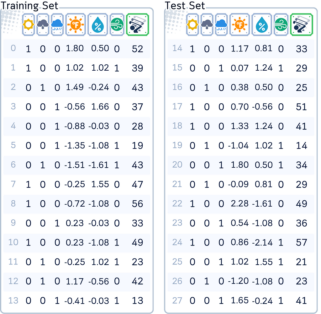
To illustrate our concepts, we’ll use our standard dataset that predicts the number of golfers visiting on a given day, using features like weather outlook, temperature, humidity, and wind conditions.
For both Lasso and Elastic Net to work effectively, we need to standardize the numerical features (making their scales comparable) and apply one-hot-encoding to categorical features, as both models’ penalties are sensitive to feature scales.
import pandas as pd
from sklearn.model_selection import train_test_split
from sklearn.preprocessing import StandardScaler
from sklearn.compose import ColumnTransformer

# Create dataset
data = {
    'Outlook': ['sunny', 'sunny', 'overcast', 'rain', 'rain', 'rain', 'overcast', 'sunny', 'sunny',
                'rain', 'sunny', 'overcast', 'overcast', 'rain', 'sunny', 'overcast', 'rain', 'sunny',
                'sunny', 'rain', 'overcast', 'rain', 'sunny', 'overcast', 'sunny', 'overcast', 'rain', 'overcast'],
    'Temperature': [85, 80, 83, 70, 68, 65, 64, 72, 69, 75, 75, 72, 81, 71, 81, 74, 76, 78, 82,
                   67, 85, 73, 88, 77, 79, 80, 66, 84],
    'Humidity': [85, 90, 78, 96, 80, 70, 65, 95, 70, 80, 70, 90, 75, 80, 88, 92, 85, 75, 92,
                 90, 85, 88, 65, 70, 60, 95, 70, 78],
    'Wind': [False, True, False, False, False, True, True, False, False, False, True, True, False,
             True, True, False, False, True, False, True, True, False, True, False, False, True, False, False],
    'Num_Players': [52, 39, 43, 37, 28, 19, 43, 47, 56, 33, 49, 23, 42, 13, 33, 29, 25, 51, 41,
                    14, 34, 29, 49, 36, 57, 21, 23, 41]
}

# Process data
df = pd.get_dummies(pd.DataFrame(data), columns=['Outlook'])
df['Wind'] = df['Wind'].astype(int)

# Split data
X, y = df.drop(columns='Num_Players'), df['Num_Players']
X_train, X_test, y_train, y_test = train_test_split(X, y, train_size=0.5, shuffle=False)

# Scale numerical features
numerical_cols = ['Temperature', 'Humidity']
ct = ColumnTransformer([('scaler', StandardScaler(), numerical_cols)], remainder='passthrough')

# Transform data
X_train_scaled = pd.DataFrame(
    ct.fit_transform(X_train),
    columns=numerical_cols + [col for col in X_train.columns if col not in numerical_cols],
    index=X_train.index
)

X_test_scaled = pd.DataFrame(
    ct.transform(X_test),
    columns=X_train_scaled.columns,
    index=X_test.index
)
Main Mechanism
Lasso and Elastic Net Regression predict numbers by making a straight line (or hyperplane) from the data, while controlling the size of coefficients in different ways:
- Both models find the best line by balancing prediction accuracy with coefficient control. They work to make the gaps between real and predicted values small, while keeping coefficients in check through penalty terms.
- In Lasso, the penalty (controlled by λ) can shrink coefficients to exactly zero, removing features entirely. Elastic Net combines two types of penalties: one that can remove features (like Lasso) and another that shrinks groups of related features together. The mix between these penalties is controlled by the l1_ratio (α).
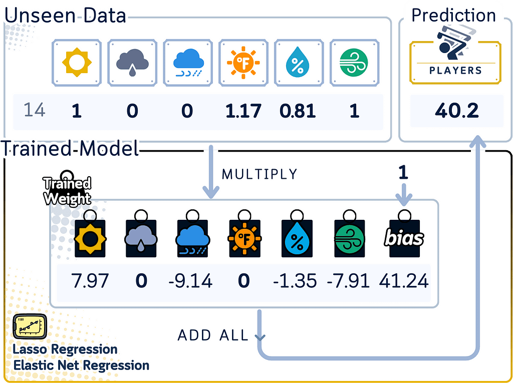
- To predict a new answer, both models multiply each input by its coefficient (if not zero) and add them up, plus a starting number (intercept/bias). Elastic Net often keeps more features than Lasso but with smaller coefficients, especially when features are correlated.
- The strength of penalties affects how the models behave:
– In Lasso, larger λ means more coefficients become zero
– In Elastic Net, λ controls overall penalty strength, while α determines the balance between feature removal and coefficient shrinkage
– When penalties are very small, both models act more like standard Linear Regression
Training Steps
Let’s explore how Lasso and Elastic Net learn from data using the coordinate descent algorithm. While these models have complex mathematical foundations, we’ll focus on understanding coordinate descent — an efficient optimization method that makes the computation more practical and intuitive.
Coordinate Descent for Lasso Regression
The optimization problem of Lasso Regression is as follows:

Here’s how coordinate descent finds the optimal coefficients by updating one feature at a time:
1. Start by initializing the model with all coefficients at zero. Set a fixed value for the regularization parameter that will control the strength of the penalty.

2. Calculate the initial bias by taking the mean of all target values.
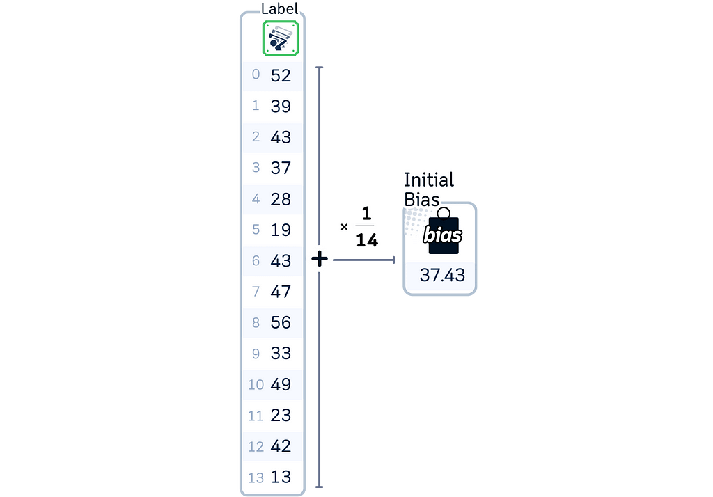
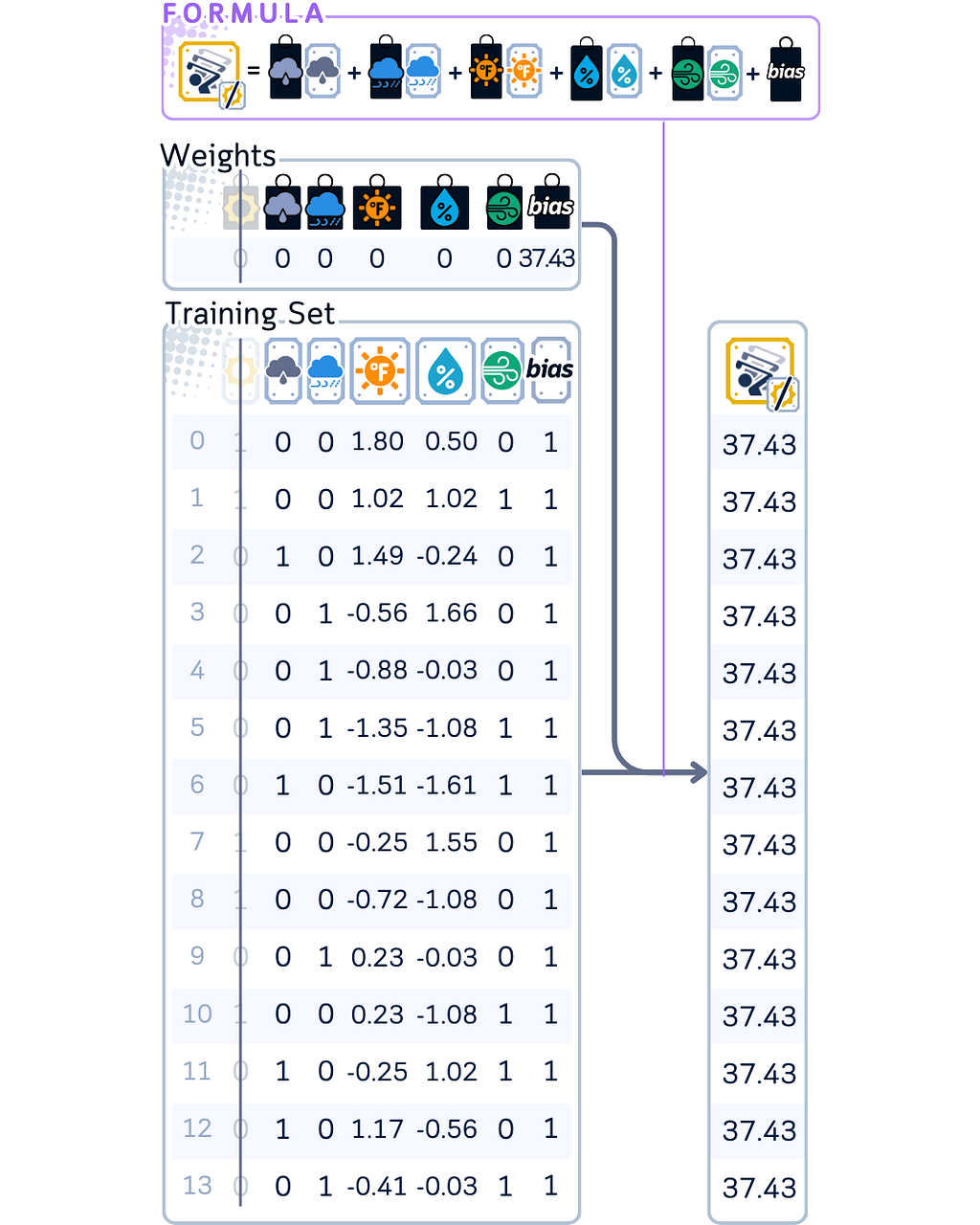
3. For updating the first coefficient (in our case, ‘sunny’):
– Using weighted sum, calculate what the model would predict without using this feature.
– Find the partial residual — how far off these predictions are from the actual values. Using this value, calculate the temporary coefficient.
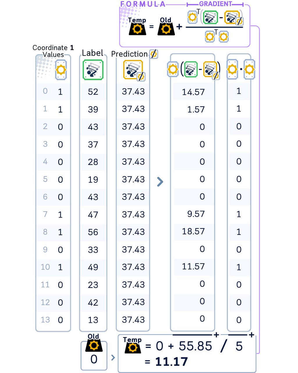
– Apply the Lasso shrinkage (soft thresholding) to this temporary coefficient to get the final coefficient for this step.
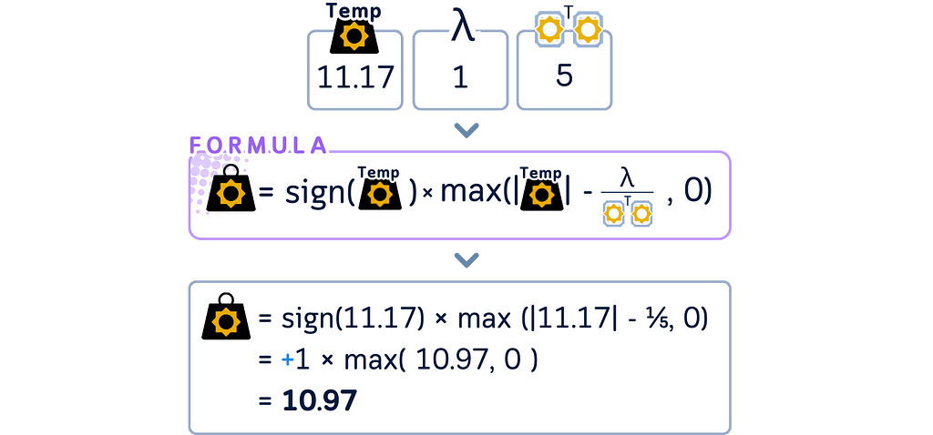
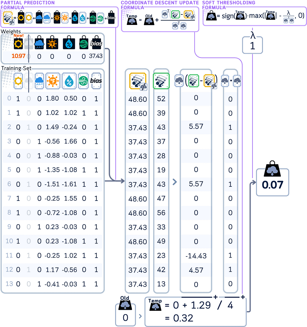
4. Move through each remaining coefficient one at a time, repeating the same update process. When calculating predictions during each update, use the most recently updated values for all other coefficients.
import numpy as np

# Initialize bias as mean of target values and coefficients to 0
bias = np.mean(y_train)
beta = np.zeros(X_train_scaled.shape[1])
lambda_param = 1

# One cycle through all features
for j, feature in enumerate(X_train_scaled.columns):
    # Get current feature values
    x_j = X_train_scaled.iloc[:, j].values

    # Calculate prediction excluding the j-th feature
    y_pred_no_j = bias + X_train_scaled.values @ beta - x_j * beta[j]

    # Calculate partial residuals
    residual_no_j = y_train.values - y_pred_no_j

    # Calculate the dot product of x_j with itself (sum of squared feature values)
    sum_squared_x_j = np.dot(x_j, x_j)

    # Calculate temporary beta without regularization (raw update)
    beta_old = beta[j]
    beta_temp = beta_old + np.dot(x_j, residual_no_j) / sum_squared_x_j

    # Apply soft thresholding for Lasso penalty
    beta[j] = np.sign(beta_temp) * max(abs(beta_temp) - lambda_param / sum_squared_x_j, 0)

# Print results
print("Coefficients after one cycle:")
for feature, coef in zip(X_train_scaled.columns, beta):
    print(f"{feature:11}: {coef:.2f}")
5. Return to update the bias by calculating what the current model predicts using all features, then adjust the bias based on the average difference between these predictions and actual values.
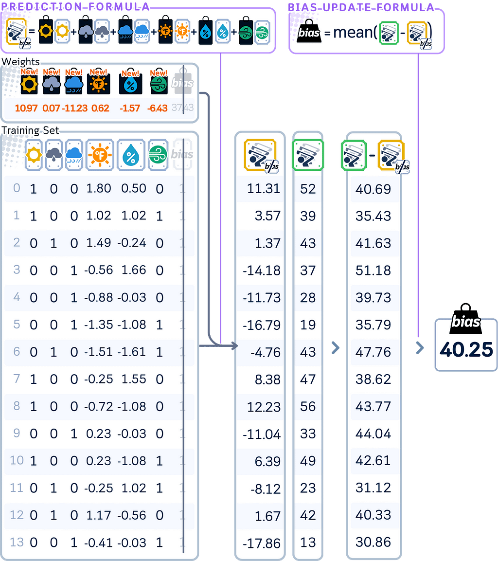
# Update bias (not penalized by lambda)
y_pred = X_train_scaled.values @ beta  # only using coefficients, no bias
residuals = y_train.values - y_pred
bias = np.mean(residuals)  # this replaces the old bias
6. Check if the model has converged either by reaching the maximum number of allowed iterations or by seeing that coefficients aren’t changing much anymore. If not converged, return to step 3 and repeat the process.

from sklearn.linear_model import Lasso

# Fit Lasso from scikit-learn
lasso = Lasso(alpha=1) # Default value is 1000 cycle
lasso.fit(X_train_scaled, y_train)

# Print results
print("nCoefficients after 1000 cycles:")
print(f"Bias term  : {lasso.intercept_:.2f}")
for feature, coef in zip(X_train_scaled.columns, lasso.coef_):
   print(f"{feature:11}: {coef:.2f}")
Coordinate Descent for Elastic Net Regression
The optimization problem of Elastic Net Regression is as follows:

The coordinate descent algorithm for Elastic Net works similarly to Lasso, but accounts for both penalties when updating coefficients. Here’s how it works:
1. Start by initializing the model with all coefficients at zero. Set two fixed values: one controlling feature removal (like in Lasso) and another for general coefficient shrinkage (the key difference from Lasso).

2. Calculate the initial bias by taking the mean of all target values. (Same as Lasso)
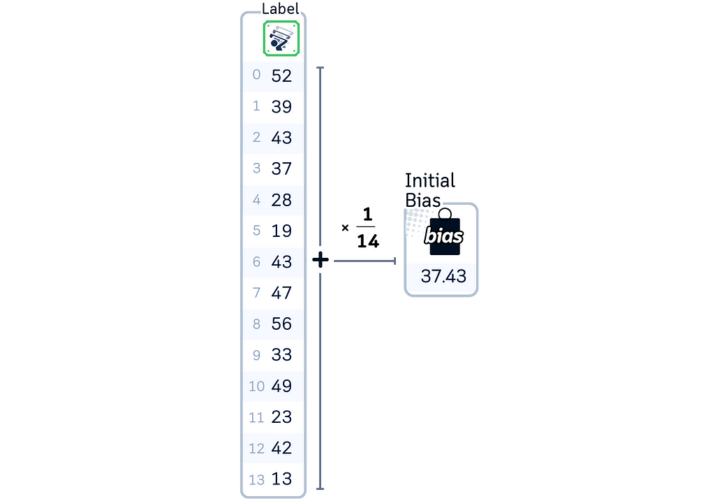
3. For updating the first coefficient:
– Using weighted sum, calculate what the model would predict without using this feature. (Same as Lasso)

– Find the partial residual — how far off these predictions are from the actual values. Using this value, calculate the temporary coefficient. (Same as Lasso)

– For Elastic Net, apply both soft thresholding and coefficient shrinkage to this temporary coefficient to get the final coefficient for this step. This combined effect is the main difference from Lasso Regression.
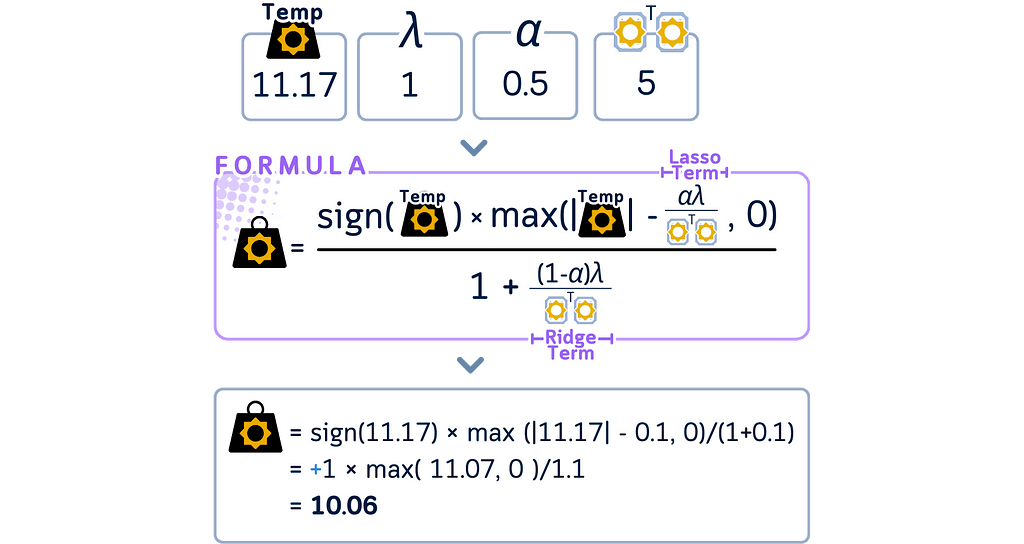
4. Move through each remaining coefficient one at a time, repeating the same update process. When calculating predictions during each update, use the most recently updated values for all other coefficients. (Same process as Lasso, but using the modified update formula)
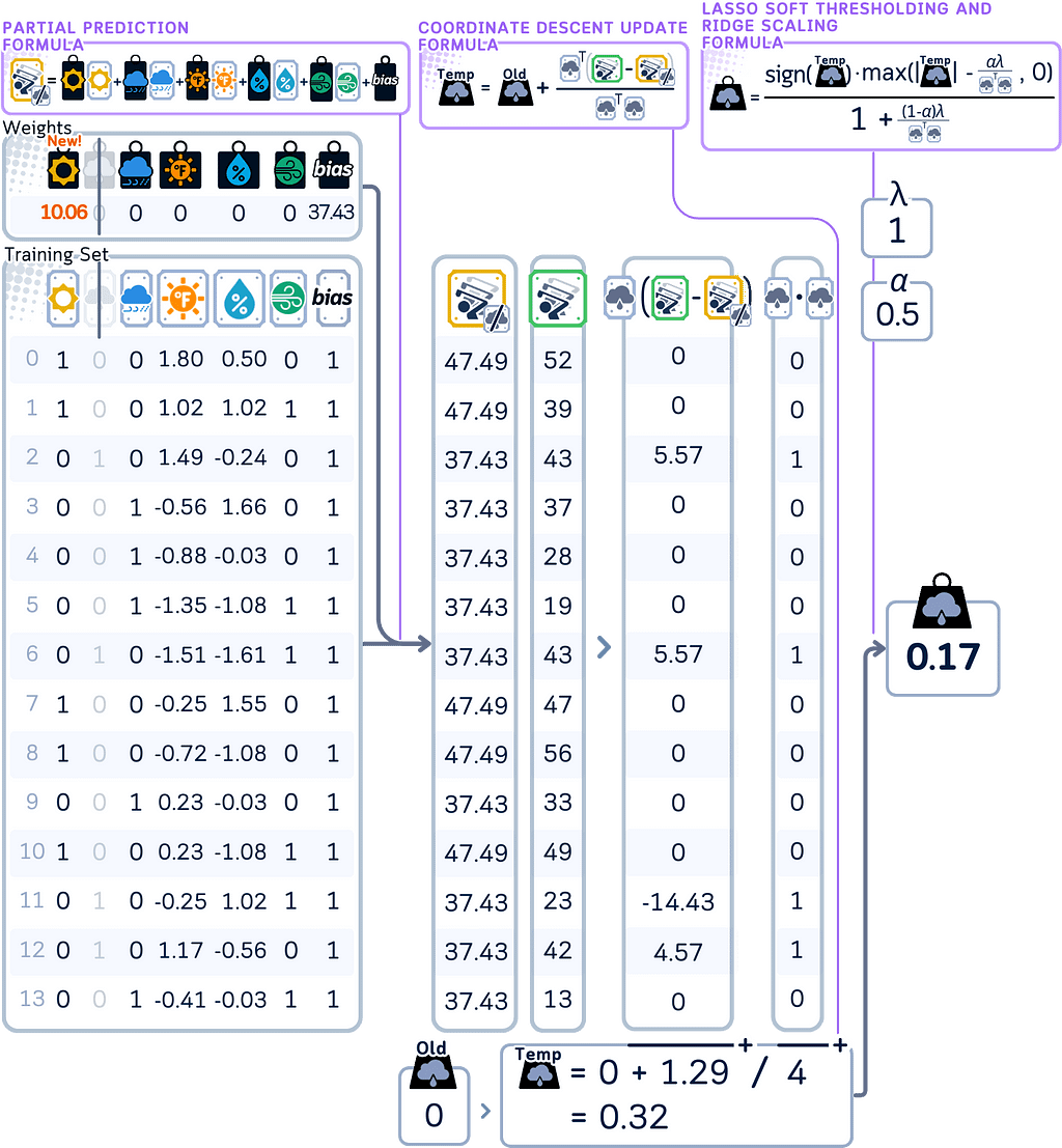
import numpy as np

# Initialize bias as mean of target values and coefficients to 0
bias = np.mean(y_train)
beta = np.zeros(X_train_scaled.shape[1])
lambda_param = 1
alpha = 0.5  # mixing parameter (0 for Ridge, 1 for Lasso)

# One cycle through all features
for j, feature in enumerate(X_train_scaled.columns):
    # Get current feature values
    x_j = X_train_scaled.iloc[:, j].values

    # Calculate prediction excluding the j-th feature
    y_pred_no_j = bias + X_train_scaled.values @ beta - x_j * beta[j]

    # Calculate partial residuals
    residual_no_j = y_train.values - y_pred_no_j

    # Calculate the dot product of x_j with itself (sum of squared feature values)
    sum_squared_x_j = np.dot(x_j, x_j)

    # Calculate temporary beta without regularization (raw update)
    beta_old = beta[j]
    beta_temp = beta_old + np.dot(x_j, residual_no_j) / sum_squared_x_j

    # Apply soft thresholding for Elastic Net penalty
    l1_term = alpha * lambda_param / sum_squared_x_j     # L1 (Lasso) penalty term
    l2_term = (1-alpha) * lambda_param / sum_squared_x_j # L2 (Ridge) penalty term

    # First apply L1 soft thresholding, then L2 scaling
    beta[j] = (np.sign(beta_temp) * max(abs(beta_temp) - l1_term, 0)) / (1 + l2_term)

# Print results
print("Coefficients after one cycle:")
for feature, coef in zip(X_train_scaled.columns, beta):
    print(f"{feature:11}: {coef:.2f}")
5. Update the bias by calculating what the current model predicts using all features, then adjust the bias based on the average difference between these predictions and actual values. (Same as Lasso)

# Update bias (not penalized by lambda)
y_pred_with_updated_beta = X_train_scaled.values @ beta  # only using coefficients, no bias
residuals_for_bias_update = y_train.values - y_pred_with_updated_beta
new_bias = np.mean(y_train.values - y_pred_with_updated_beta)  # this replaces the old bias

print(f"Bias term  : {new_bias:.2f}")
6. Check if the model has converged either by reaching the maximum number of allowed iterations or by seeing that coefficients aren’t changing much anymore. If not converged, return to step 3 and repeat the process.

from sklearn.linear_model import ElasticNet

# Fit Lasso from scikit-learn
elasticnet = Lasso(alpha=1) # Default value is 1000 cycle
elasticnet.fit(X_train_scaled, y_train)

# Print results
print("nCoefficients after 1000 cycles:")
print(f"Bias term  : {elasticnet.intercept_:.2f}")
for feature, coef in zip(X_train_scaled.columns, elasticnet.coef_):
   print(f"{feature:11}: {coef:.2f}")
Test Step
The prediction process remains the same as OLS — multiply new data points by the coefficients:
Lasso Regression
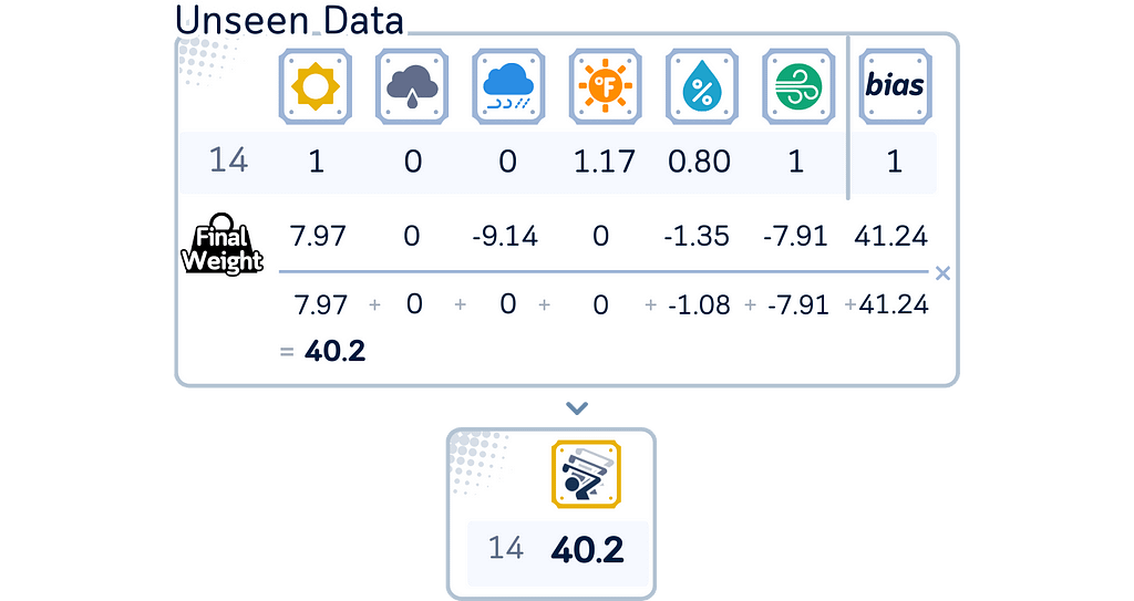
Elastic Net Regression
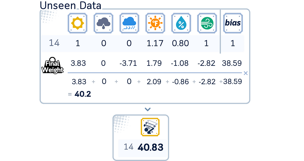
Evaluation Step
We can do the same process for all data points. For our dataset, here’s the final result with the RMSE as well:
Lasso Regression
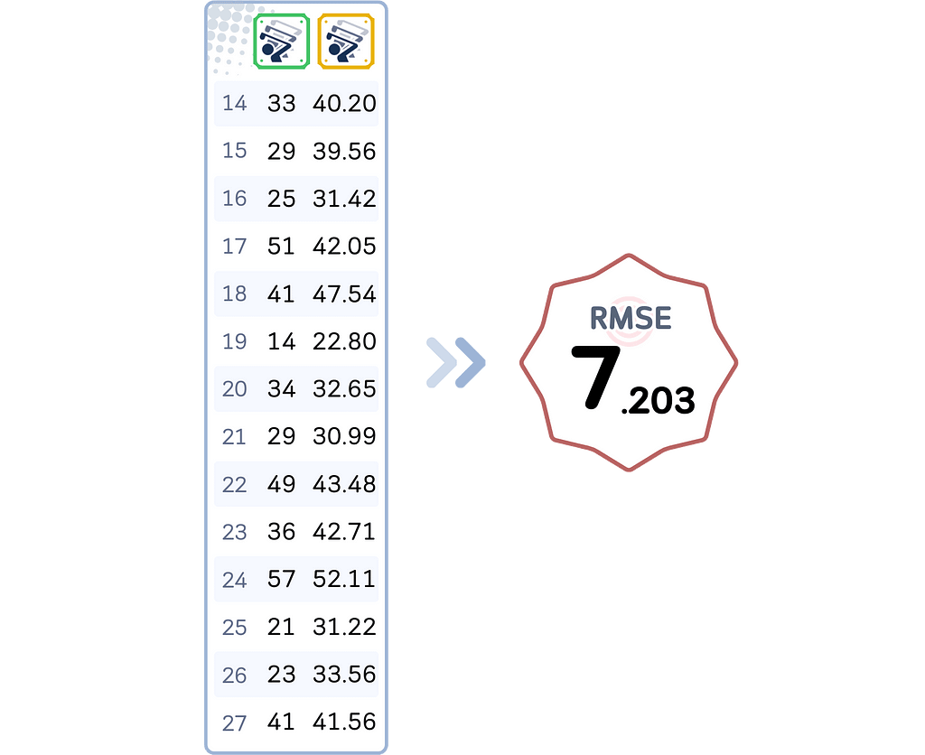
Elastic Net Regression

Key Parameters
Lasso Regression
Lasso regression uses coordinate descent to solve the optimization problem. Here are the key parameters for that:
- alpha (λ): Controls how strongly to penalize large coefficients. Higher values force more coefficients to become exactly zero. Default is 1.0.
- max_iter: Sets the maximum number of cycles the algorithm will update its solution in search of the best result. Default is 1000.
- tol: Sets how small the change in coefficients needs to be before the algorithm decides it has found a good enough solution. Default is 0.0001.
Elastic Net Regression
Elastic Net regression combines two types of penalties and also uses coordinate descent. Here are the key parameters for that:
- alpha (λ): Controls the overall strength of both penalties together. Higher values mean stronger penalties. Default is 1.0.
- l1_ratio (α): Sets how much to use each type of penalty. A value of 0 uses only Ridge penalty, while 1 uses only Lasso penalty. Values between 0 and 1 use both. Default is 0.5.
- max_iter: Maximum number of iterations for the coordinate descent algorithm. Default is 1000 iterations.
- tol: Tolerance for the optimization convergence, similar to Lasso. Default is 1e-4.
Note: Not to be confused, in scikit-learn’s code, the regularization parameter is called alpha, but in mathematical notation it’s typically written as λ (lambda). Similarly, the mixing parameter is called l1_ratio in code but written as α (alpha) in mathematical notation. We use the mathematical symbols here to match standard textbook notation.
Model Comparison: OLS vs Lasso vs Ridge vs Elastic Net
With Elastic Net, we can actually explore different types of linear regression models by adjusting the parameters:
- When alpha = 0, we get Ordinary Least Squares (OLS)
- When alpha > 0 and l1_ratio = 0, we get Ridge regression
- When alpha > 0 and l1_ratio = 1, we get Lasso regression
- When alpha > 0 and 0 < l1_ratio < 1, we get Elastic Net regression
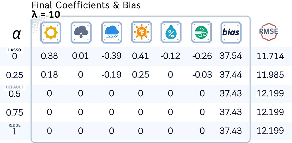
In practice, it is a good idea to explore a range of alpha values (like 0.0001, 0.001, 0.01, 0.1, 1, 10, 100) and l1_ratio values (like 0, 0.25, 0.5, 0.75, 1), preferably using cross-validation to find the best combination.
Here, let’s see how the model coefficients, bias terms, and test RMSE change with different regularization strengths (λ) and mixing parameters (l1_ratio).


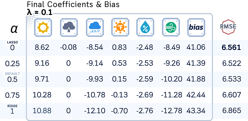
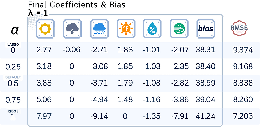
# Define parameters
l1_ratios = [0, 0.25, 0.5, 0.75, 1]
lambdas = [0, 0.01, 0.1, 1, 10]
feature_names = X_train_scaled.columns

# Create a dataframe for each lambda value
for lambda_val in lambdas:
    # Initialize list to store results
    results = []
    rmse_values = []

    # Fit ElasticNet for each l1_ratio
    for l1_ratio in l1_ratios:
        # Fit model
        en = ElasticNet(alpha=lambda_val, l1_ratio=l1_ratio)
        en.fit(X_train_scaled, y_train)

        # Calculate RMSE
        y_pred = en.predict(X_test_scaled)
        rmse = root_mean_squared_error(y_test, y_pred)

        # Store coefficients and RMSE
        results.append(list(en.coef_.round(2)) + [round(en.intercept_,2),round(rmse,3)])

    # Create dataframe with RMSE column
    columns = list(feature_names) + ['Bias','RMSE']
    df = pd.DataFrame(results, index=l1_ratios, columns=columns)
    df.index.name = f'λ = {lambda_val}'

    print(df)
Note: Even though Elastic Net can do what OLS, Ridge, and Lasso do by changing its parameters, it’s better to use the specific command made for each type of regression. In scikit-learn, use LinearRegression for OLS, Ridge for Ridge regression, and Lasso for Lasso regression. Only use Elastic Net when you want to combine both Lasso and Ridge’s special features together.
Final Remarks: Which Regression Method Should You Use?
Let’s break down when to use each method.
Start with Ordinary Least Squares (OLS) when you have more samples than features in your dataset, and when your features don’t strongly predict each other.
Ridge Regression works well when you have the opposite situation — lots of features compared to your number of samples. It’s also great when your features are strongly connected to each other.
Lasso Regression is best when you want to discover which features actually matter for your predictions. It will automatically set unimportant features to zero, making your model simpler.
Elastic Net combines the strengths of both Ridge and Lasso. It’s useful when you have groups of related features and want to either keep or remove them together. If you’ve tried Ridge and Lasso separately and weren’t happy with the results, Elastic Net might give you better predictions.
A good strategy is to start with Ridge if you want to keep all your features. You can move on to Lasso if you want to identify the important ones. If neither gives you good results, then move on to Elastic Net.
🌟 Lasso and Elastic Net Code Summarized
import pandas as pd
from sklearn.model_selection import train_test_split
from sklearn.preprocessing import StandardScaler
from sklearn.compose import ColumnTransformer
from sklearn.metrics import root_mean_squared_error
from sklearn.linear_model import Lasso  #, ElasticNet

# Create dataset
data = {
    'Outlook': ['sunny', 'sunny', 'overcast', 'rain', 'rain', 'rain', 'overcast', 'sunny', 'sunny',
                'rain', 'sunny', 'overcast', 'overcast', 'rain', 'sunny', 'overcast', 'rain', 'sunny',
                'sunny', 'rain', 'overcast', 'rain', 'sunny', 'overcast', 'sunny', 'overcast', 'rain', 'overcast'],
    'Temperature': [85, 80, 83, 70, 68, 65, 64, 72, 69, 75, 75, 72, 81, 71, 81, 74, 76, 78, 82,
                   67, 85, 73, 88, 77, 79, 80, 66, 84],
    'Humidity': [85, 90, 78, 96, 80, 70, 65, 95, 70, 80, 70, 90, 75, 80, 88, 92, 85, 75, 92,
                 90, 85, 88, 65, 70, 60, 95, 70, 78],
    'Wind': [False, True, False, False, False, True, True, False, False, False, True, True, False,
             True, True, False, False, True, False, True, True, False, True, False, False, True, False, False],
    'Num_Players': [52, 39, 43, 37, 28, 19, 43, 47, 56, 33, 49, 23, 42, 13, 33, 29, 25, 51, 41,
                    14, 34, 29, 49, 36, 57, 21, 23, 41]
}

# Process data
df = pd.get_dummies(pd.DataFrame(data), columns=['Outlook'], prefix='', prefix_sep='', dtype=int)
df['Wind'] = df['Wind'].astype(int)
df = df[['sunny','overcast','rain','Temperature','Humidity','Wind','Num_Players']]

# Split data
X, y = df.drop(columns='Num_Players'), df['Num_Players']
X_train, X_test, y_train, y_test = train_test_split(X, y, train_size=0.5, shuffle=False)

# Scale numerical features
numerical_cols = ['Temperature', 'Humidity']
ct = ColumnTransformer([('scaler', StandardScaler(), numerical_cols)], remainder='passthrough')

# Transform data
X_train_scaled = pd.DataFrame(
    ct.fit_transform(X_train),
    columns=numerical_cols + [col for col in X_train.columns if col not in numerical_cols],
    index=X_train.index
)
X_test_scaled = pd.DataFrame(
    ct.transform(X_test),
    columns=X_train_scaled.columns,
    index=X_test.index
)

# Initialize and train the model
model = Lasso(alpha=0.1)  # Option 1: Lasso Regression (alpha is the regularization strength, equivalent to λ, uses coordinate descent)
#model = ElasticNet(alpha=0.1, l1_ratio=0.5)  # Option 2: Elastic Net Regression (alpha is the overall regularization strength, and l1_ratio is the mix between L1 and L2, uses coordinate descent)

# Fit the model
model.fit(X_train_scaled, y_train)

# Make predictions
y_pred = model.predict(X_test_scaled)

# Calculate and print RMSE
rmse = root_mean_squared_error(y_test, y_pred)
print(f"RMSE: {rmse:.4f}")

# Additional information about the model
print("nModel Coefficients:")
for feature, coef in zip(X_train_scaled.columns, model.coef_):
    print(f"{feature:13}: {coef:.2f}")
print(f"Intercept    : {model.intercept_:.2f}")
Further Reading
For a detailed explanation of Lasso Regression and Elastic Net Regression, and its implementation in scikit-learn, readers can refer to their official documentation. It provides comprehensive information on their usage and parameters.
Technical Environment
This article uses Python 3.7 and scikit-learn 1.5. While the concepts discussed are generally applicable, specific code implementations may vary slightly with different versions
About the Illustrations
Unless otherwise noted, all images are created by the author, incorporating licensed design elements from Canva Pro.
𝙎𝙚𝙚 𝙢𝙤𝙧𝙚 𝙍𝙚𝙜𝙧𝙚𝙨𝙨𝙞𝙤𝙣 𝘼𝙡𝙜𝙤𝙧𝙞𝙩𝙝𝙢𝙨 𝙝𝙚𝙧𝙚:
𝙔𝙤𝙪 𝙢𝙞𝙜𝙝𝙩 𝙖𝙡𝙨𝙤 𝙡𝙞𝙠𝙚:
Lasso and Elastic Net Regressions, Explained: A Visual Guide with Code Examples was originally published in Towards Data Science on Medium, where people are continuing the conversation by highlighting and responding to this story.
REGRESSION ALGORITHMRoping in key features with coordinate descentLeast Squares Regression, Explained: A Visual Guide with Code Examples for BeginnersLinear regression comes in different types: Least Squares methods form the foundation, from the classic Ordinary Least Squares (OLS) to Ridge regression with its regularization to prevent overfitting. Then there’s Lasso regression, which takes a unique approach by automatically selecting important factors and ignoring others. Elastic Net combines the best of both worlds, mixing Lasso’s feature selection with Ridge’s ability to handle related features.It’s frustrating to see many articles treat these methods as if they’re basically the same thing with minor tweaks. They make it seem like switching between them is as simple as changing a setting in your code, but each actually uses different approaches to solve their optimization problems!While OLS and Ridge regression can be solved directly through matrix operations, Lasso and Elastic Net require a different approach — an iterative method called coordinate descent. Here, we’ll explore how this algorithm works through clear visualizations. So, let’s saddle up and lasso our way through the details!All visuals: Author-created using Canva Pro. Optimized for mobile; may appear oversized on desktop.DefinitionLasso RegressionLASSO (Least Absolute Shrinkage and Selection Operator) is a variation of Linear Regression that adds a penalty to the model. It uses a linear equation to predict numbers, just like Linear Regression. However, Lasso also has a way to reduce the importance of certain factors to zero, which makes it useful for two main tasks: making predictions and identifying the most important features.Elastic Net RegressionElastic Net Regression is a mix of Ridge and Lasso Regression that combines their penalty terms. The name “Elastic Net” comes from physics: just like an elastic net can stretch and still keep its shape, this method adapts to data while maintaining structure.The model balances three goals: minimizing prediction errors, keeping the size of coefficients small (like Lasso), and preventing any coefficient from becoming too large (like Ridge). To use the model, you input your data’s feature values into the linear equation, just like in standard Linear Regression.The main advantage of Elastic Net is that when features are related, it tends to keep or remove them as a group instead of randomly picking one feature from the group.Linear models like Lasso and Elastic Net belong to the broader family of machine learning methods that predict outcomes using linear relationships between variables.📊 Dataset UsedTo illustrate our concepts, we’ll use our standard dataset that predicts the number of golfers visiting on a given day, using features like weather outlook, temperature, humidity, and wind conditions.For both Lasso and Elastic Net to work effectively, we need to standardize the numerical features (making their scales comparable) and apply one-hot-encoding to categorical features, as both models’ penalties are sensitive to feature scales.Columns: ‘Outlook’ (one-hot encoded to sunny, overcast, rain), ‘Temperature’ (standardized), ‘Humidity’ (standardized), ‘Wind’ (Yes/No) and ‘Number of Players’ (numerical, target feature)import pandas as pdfrom sklearn.model_selection import train_test_splitfrom sklearn.preprocessing import StandardScalerfrom sklearn.compose import ColumnTransformer# Create datasetdata = { ‘Outlook’: [‘sunny’, ‘sunny’, ‘overcast’, ‘rain’, ‘rain’, ‘rain’, ‘overcast’, ‘sunny’, ‘sunny’, ‘rain’, ‘sunny’, ‘overcast’, ‘overcast’, ‘rain’, ‘sunny’, ‘overcast’, ‘rain’, ‘sunny’, ‘sunny’, ‘rain’, ‘overcast’, ‘rain’, ‘sunny’, ‘overcast’, ‘sunny’, ‘overcast’, ‘rain’, ‘overcast’], ‘Temperature’: [85, 80, 83, 70, 68, 65, 64, 72, 69, 75, 75, 72, 81, 71, 81, 74, 76, 78, 82, 67, 85, 73, 88, 77, 79, 80, 66, 84], ‘Humidity’: [85, 90, 78, 96, 80, 70, 65, 95, 70, 80, 70, 90, 75, 80, 88, 92, 85, 75, 92, 90, 85, 88, 65, 70, 60, 95, 70, 78], ‘Wind’: [False, True, False, False, False, True, True, False, False, False, True, True, False, True, True, False, False, True, False, True, True, False, True, False, False, True, False, False], ‘Num_Players’: [52, 39, 43, 37, 28, 19, 43, 47, 56, 33, 49, 23, 42, 13, 33, 29, 25, 51, 41, 14, 34, 29, 49, 36, 57, 21, 23, 41]}# Process datadf = pd.get_dummies(pd.DataFrame(data), columns=[‘Outlook’])df[‘Wind’] = df[‘Wind’].astype(int)# Split dataX, y = df.drop(columns=’Num_Players’), df[‘Num_Players’]X_train, X_test, y_train, y_test = train_test_split(X, y, train_size=0.5, shuffle=False)# Scale numerical featuresnumerical_cols = [‘Temperature’, ‘Humidity’]ct = ColumnTransformer([(‘scaler’, StandardScaler(), numerical_cols)], remainder=’passthrough’)# Transform dataX_train_scaled = pd.DataFrame( ct.fit_transform(X_train), columns=numerical_cols + [col for col in X_train.columns if col not in numerical_cols], index=X_train.index)X_test_scaled = pd.DataFrame( ct.transform(X_test), columns=X_train_scaled.columns, index=X_test.index)Main MechanismLasso and Elastic Net Regression predict numbers by making a straight line (or hyperplane) from the data, while controlling the size of coefficients in different ways:Both models find the best line by balancing prediction accuracy with coefficient control. They work to make the gaps between real and predicted values small, while keeping coefficients in check through penalty terms.In Lasso, the penalty (controlled by λ) can shrink coefficients to exactly zero, removing features entirely. Elastic Net combines two types of penalties: one that can remove features (like Lasso) and another that shrinks groups of related features together. The mix between these penalties is controlled by the l1_ratio (α).To predict a new answer, both models multiply each input by its coefficient (if not zero) and add them up, plus a starting number (intercept/bias). Elastic Net often keeps more features than Lasso but with smaller coefficients, especially when features are correlated.The strength of penalties affects how the models behave:- In Lasso, larger λ means more coefficients become zero- In Elastic Net, λ controls overall penalty strength, while α determines the balance between feature removal and coefficient shrinkage- When penalties are very small, both models act more like standard Linear RegressionLasso and Elastic Net make predictions by multiplying input features with their trained weights and adding them together with a bias term to produce a final output value.Training StepsLet’s explore how Lasso and Elastic Net learn from data using the coordinate descent algorithm. While these models have complex mathematical foundations, we’ll focus on understanding coordinate descent — an efficient optimization method that makes the computation more practical and intuitive.Coordinate Descent for Lasso RegressionThe optimization problem of Lasso Regression is as follows:While scikit-learn implementation includes additional scaling factors (1/(2*n_samples)) for computational efficiency, we’ll use the standard theoretical form for clarity in our explanation.Here’s how coordinate descent finds the optimal coefficients by updating one feature at a time:1. Start by initializing the model with all coefficients at zero. Set a fixed value for the regularization parameter that will control the strength of the penalty.Lasso regression begins with all feature weights set to zero and uses a penalty parameter (λ) to control how much it shrinks weights during training.2. Calculate the initial bias by taking the mean of all target values.The initial bias value is set to 37.43, which is calculated by taking the average of all target values in the training data (mean of player counts shown from index 0 to 13).3. For updating the first coefficient (in our case, ‘sunny’): – Using weighted sum, calculate what the model would predict without using this feature.At the start of training, all feature weights are set to zero while using the initial bias of 37.43, causing the model to predict the same average value (37.43) for all training examples regardless of their input features.- Find the partial residual — how far off these predictions are from the actual values. Using this value, calculate the temporary coefficient.For the first feature, Lasso calculates a temporary coefficient of 11.17 by comparing the true labels with predictions, considering only the rows where this feature equals 1, and applying the gradient formula.- Apply the Lasso shrinkage (soft thresholding) to this temporary coefficient to get the final coefficient for this step.Lasso applies its shrinkage formula to the temporary coefficient (11.17), where it subtracts the penalty term (λ/5 = 0.2) from the absolute value while preserving the sign, resulting in a final coefficient of 10.97.4. Move through each remaining coefficient one at a time, repeating the same update process. When calculating predictions during each update, use the most recently updated values for all other coefficients.After updating the first coefficient to 10.97, Lasso uses these updated predictions to calculate the temporary coefficient (0.32) for the second feature, showing how the algorithm updates coefficients one at a time through coordinate descent.import numpy as np# Initialize bias as mean of target values and coefficients to 0bias = np.mean(y_train)beta = np.zeros(X_train_scaled.shape[1])lambda_param = 1# One cycle through all featuresfor j, feature in enumerate(X_train_scaled.columns): # Get current feature values x_j = X_train_scaled.iloc[:, j].values # Calculate prediction excluding the j-th feature y_pred_no_j = bias + X_train_scaled.values @ beta – x_j * beta[j] # Calculate partial residuals residual_no_j = y_train.values – y_pred_no_j # Calculate the dot product of x_j with itself (sum of squared feature values) sum_squared_x_j = np.dot(x_j, x_j) # Calculate temporary beta without regularization (raw update) beta_old = beta[j] beta_temp = beta_old + np.dot(x_j, residual_no_j) / sum_squared_x_j # Apply soft thresholding for Lasso penalty beta[j] = np.sign(beta_temp) * max(abs(beta_temp) – lambda_param / sum_squared_x_j, 0)# Print resultsprint(“Coefficients after one cycle:”)for feature, coef in zip(X_train_scaled.columns, beta): print(f”{feature:11}: {coef:.2f}”)5. Return to update the bias by calculating what the current model predicts using all features, then adjust the bias based on the average difference between these predictions and actual values.After updating all feature coefficients through coordinate descent, the model recalculates the bias (40.25) as the mean difference between the true labels and the predictions made using the current feature weights, ensuring the model’s predictions are properly centered around the target values.# Update bias (not penalized by lambda)y_pred = X_train_scaled.values @ beta # only using coefficients, no biasresiduals = y_train.values – y_predbias = np.mean(residuals) # this replaces the old bias6. Check if the model has converged either by reaching the maximum number of allowed iterations or by seeing that coefficients aren’t changing much anymore. If not converged, return to step 3 and repeat the process.After 1000 iterations of coordinate descent, Lasso produces the final model where some coefficients have been shrunk exactly to zero (‘rain’ and ‘Temperature’ features), while others retain non-zero values, demonstrating Lasso’s feature selection capability.from sklearn.linear_model import Lasso# Fit Lasso from scikit-learnlasso = Lasso(alpha=1) # Default value is 1000 cyclelasso.fit(X_train_scaled, y_train)# Print resultsprint(“nCoefficients after 1000 cycles:”)print(f”Bias term : {lasso.intercept_:.2f}”)for feature, coef in zip(X_train_scaled.columns, lasso.coef_): print(f”{feature:11}: {coef:.2f}”)Coordinate Descent for Elastic Net RegressionThe optimization problem of Elastic Net Regression is as follows:While scikit-learn’s implementation includes additional scaling factors (1/(2*n_samples)) and uses alpha (α) to control overall regularization strength and l1_ratio to control the penalty mix, we’ll use the standard theoretical form for clarity.The coordinate descent algorithm for Elastic Net works similarly to Lasso, but accounts for both penalties when updating coefficients. Here’s how it works:1. Start by initializing the model with all coefficients at zero. Set two fixed values: one controlling feature removal (like in Lasso) and another for general coefficient shrinkage (the key difference from Lasso).Elastic Net regression starts like Lasso with zero weights for all features, but uses two parameters: λ (lambda) for overall regularization strength and α (alpha) to balance between Lasso and Ridge penalties.2. Calculate the initial bias by taking the mean of all target values. (Same as Lasso)ike Lasso, Elastic Net also initializes its bias term to 37.43 by calculating the mean of all target values in the training dataset.3. For updating the first coefficient:- Using weighted sum, calculate what the model would predict without using this feature. (Same as Lasso)Elastic Net starts its coordinate descent process similar to Lasso, making initial predictions of 37.43 for all training examples since all feature weights are set to zero and only the bias term is active.- Find the partial residual — how far off these predictions are from the actual values. Using this value, calculate the temporary coefficient. (Same as Lasso)Like Lasso, Elastic Net calculates a temporary coefficient of 11.17 for the first feature by comparing predictions with true labels.- For Elastic Net, apply both soft thresholding and coefficient shrinkage to this temporary coefficient to get the final coefficient for this step. This combined effect is the main difference from Lasso Regression.Elastic Net applies its unique shrinkage formula that combines both Lasso (L1) and Ridge (L2) penalties, where α controls their balance. The temporary coefficient 11.17 is shrunk to 10.06 through this combined regularization approach.4. Move through each remaining coefficient one at a time, repeating the same update process. When calculating predictions during each update, use the most recently updated values for all other coefficients. (Same process as Lasso, but using the modified update formula)After updating the first coefficient to 10.06, Elastic Net continues coordinate descent by calculating and updating the second coefficient, showing how it processes features one at a time while maintaining both L1 and L2 regularization effects.import numpy as np# Initialize bias as mean of target values and coefficients to 0bias = np.mean(y_train)beta = np.zeros(X_train_scaled.shape[1])lambda_param = 1alpha = 0.5 # mixing parameter (0 for Ridge, 1 for Lasso)# One cycle through all featuresfor j, feature in enumerate(X_train_scaled.columns): # Get current feature values x_j = X_train_scaled.iloc[:, j].values # Calculate prediction excluding the j-th feature y_pred_no_j = bias + X_train_scaled.values @ beta – x_j * beta[j] # Calculate partial residuals residual_no_j = y_train.values – y_pred_no_j # Calculate the dot product of x_j with itself (sum of squared feature values) sum_squared_x_j = np.dot(x_j, x_j) # Calculate temporary beta without regularization (raw update) beta_old = beta[j] beta_temp = beta_old + np.dot(x_j, residual_no_j) / sum_squared_x_j # Apply soft thresholding for Elastic Net penalty l1_term = alpha * lambda_param / sum_squared_x_j # L1 (Lasso) penalty term l2_term = (1-alpha) * lambda_param / sum_squared_x_j # L2 (Ridge) penalty term # First apply L1 soft thresholding, then L2 scaling beta[j] = (np.sign(beta_temp) * max(abs(beta_temp) – l1_term, 0)) / (1 + l2_term)# Print resultsprint(“Coefficients after one cycle:”)for feature, coef in zip(X_train_scaled.columns, beta): print(f”{feature:11}: {coef:.2f}”)5. Update the bias by calculating what the current model predicts using all features, then adjust the bias based on the average difference between these predictions and actual values. (Same as Lasso)After updating all feature coefficients using Elastic Net’s combined L1 and L2 regularization, the model recalculates the bias to 40.01 by taking the mean difference between true labels and predictions, similar to the process in Lasso regression.# Update bias (not penalized by lambda)y_pred_with_updated_beta = X_train_scaled.values @ beta # only using coefficients, no biasresiduals_for_bias_update = y_train.values – y_pred_with_updated_betanew_bias = np.mean(y_train.values – y_pred_with_updated_beta) # this replaces the old biasprint(f”Bias term : {new_bias:.2f}”)6. Check if the model has converged either by reaching the maximum number of allowed iterations or by seeing that coefficients aren’t changing much anymore. If not converged, return to step 3 and repeat the process.The final Elastic Net model after 1000 iterations shows smaller coefficient values compared to Lasso and fewer coefficients shrunk exactly to zero.from sklearn.linear_model import ElasticNet# Fit Lasso from scikit-learnelasticnet = Lasso(alpha=1) # Default value is 1000 cycleelasticnet.fit(X_train_scaled, y_train)# Print resultsprint(“nCoefficients after 1000 cycles:”)print(f”Bias term : {elasticnet.intercept_:.2f}”)for feature, coef in zip(X_train_scaled.columns, elasticnet.coef_): print(f”{feature:11}: {coef:.2f}”)Test StepThe prediction process remains the same as OLS — multiply new data points by the coefficients:Lasso RegressionWhen applying the trained Lasso model to unseen data, it multiplies each feature value with its corresponding coefficient and adds the bias term (41.24), resulting in a final prediction of 40.2 players for this new data point.Elastic Net RegressionThe trained Elastic Net model predicts 40.83 players for the same unseen data point by multiplying features with its more evenly distributed coefficients and adding the bias (38.59), showing a slightly different prediction from Lasso due to its balanced regularization approach.Evaluation StepWe can do the same process for all data points. For our dataset, here’s the final result with the RMSE as well:Lasso RegressionLasso’s performance on multiple test cases shows a Root Mean Square Error (RMSE) of 7.203, calculated by comparing its predictions with actual player counts across 14 different test samples.Elastic Net RegressionElastic Net shows a slightly higher RMSE compared to Lasso’s, likely because its combined L1 and L2 penalties keep more features with small non-zero coefficients, which can introduce more variance in predictions.Key ParametersLasso RegressionLasso regression uses coordinate descent to solve the optimization problem. Here are the key parameters for that:alpha (λ): Controls how strongly to penalize large coefficients. Higher values force more coefficients to become exactly zero. Default is 1.0.max_iter: Sets the maximum number of cycles the algorithm will update its solution in search of the best result. Default is 1000.tol: Sets how small the change in coefficients needs to be before the algorithm decides it has found a good enough solution. Default is 0.0001.Elastic Net RegressionElastic Net regression combines two types of penalties and also uses coordinate descent. Here are the key parameters for that:alpha (λ): Controls the overall strength of both penalties together. Higher values mean stronger penalties. Default is 1.0.l1_ratio (α): Sets how much to use each type of penalty. A value of 0 uses only Ridge penalty, while 1 uses only Lasso penalty. Values between 0 and 1 use both. Default is 0.5.max_iter: Maximum number of iterations for the coordinate descent algorithm. Default is 1000 iterations.tol: Tolerance for the optimization convergence, similar to Lasso. Default is 1e-4.Note: Not to be confused, in scikit-learn’s code, the regularization parameter is called alpha, but in mathematical notation it’s typically written as λ (lambda). Similarly, the mixing parameter is called l1_ratio in code but written as α (alpha) in mathematical notation. We use the mathematical symbols here to match standard textbook notation.Model Comparison: OLS vs Lasso vs Ridge vs Elastic NetWith Elastic Net, we can actually explore different types of linear regression models by adjusting the parameters:When alpha = 0, we get Ordinary Least Squares (OLS)When alpha > 0 and l1_ratio = 0, we get Ridge regressionWhen alpha > 0 and l1_ratio = 1, we get Lasso regressionWhen alpha > 0 and 0 < l1_ratio < 1, we get Elastic Net regressionIn practice, it is a good idea to explore a range of alpha values (like 0.0001, 0.001, 0.01, 0.1, 1, 10, 100) and l1_ratio values (like 0, 0.25, 0.5, 0.75, 1), preferably using cross-validation to find the best combination.Here, let’s see how the model coefficients, bias terms, and test RMSE change with different regularization strengths (λ) and mixing parameters (l1_ratio).The best model is Lasso (α = 0) with λ = 0.1, achieving an RMSE of 6.561, showing that pure L1 regularization works best for our dataset.# Define parametersl1_ratios = [0, 0.25, 0.5, 0.75, 1]lambdas = [0, 0.01, 0.1, 1, 10]feature_names = X_train_scaled.columns# Create a dataframe for each lambda valuefor lambda_val in lambdas: # Initialize list to store results results = [] rmse_values = [] # Fit ElasticNet for each l1_ratio for l1_ratio in l1_ratios: # Fit model en = ElasticNet(alpha=lambda_val, l1_ratio=l1_ratio) en.fit(X_train_scaled, y_train) # Calculate RMSE y_pred = en.predict(X_test_scaled) rmse = root_mean_squared_error(y_test, y_pred) # Store coefficients and RMSE results.append(list(en.coef_.round(2)) + [round(en.intercept_,2),round(rmse,3)]) # Create dataframe with RMSE column columns = list(feature_names) + [‘Bias’,’RMSE’] df = pd.DataFrame(results, index=l1_ratios, columns=columns) df.index.name = f’λ = {lambda_val}’ print(df)Note: Even though Elastic Net can do what OLS, Ridge, and Lasso do by changing its parameters, it’s better to use the specific command made for each type of regression. In scikit-learn, use LinearRegression for OLS, Ridge for Ridge regression, and Lasso for Lasso regression. Only use Elastic Net when you want to combine both Lasso and Ridge’s special features together.Final Remarks: Which Regression Method Should You Use?Let’s break down when to use each method.Start with Ordinary Least Squares (OLS) when you have more samples than features in your dataset, and when your features don’t strongly predict each other.Ridge Regression works well when you have the opposite situation — lots of features compared to your number of samples. It’s also great when your features are strongly connected to each other.Lasso Regression is best when you want to discover which features actually matter for your predictions. It will automatically set unimportant features to zero, making your model simpler.Elastic Net combines the strengths of both Ridge and Lasso. It’s useful when you have groups of related features and want to either keep or remove them together. If you’ve tried Ridge and Lasso separately and weren’t happy with the results, Elastic Net might give you better predictions.A good strategy is to start with Ridge if you want to keep all your features. You can move on to Lasso if you want to identify the important ones. If neither gives you good results, then move on to Elastic Net.🌟 Lasso and Elastic Net Code Summarizedimport pandas as pdfrom sklearn.model_selection import train_test_splitfrom sklearn.preprocessing import StandardScalerfrom sklearn.compose import ColumnTransformerfrom sklearn.metrics import root_mean_squared_errorfrom sklearn.linear_model import Lasso #, ElasticNet# Create datasetdata = { ‘Outlook’: [‘sunny’, ‘sunny’, ‘overcast’, ‘rain’, ‘rain’, ‘rain’, ‘overcast’, ‘sunny’, ‘sunny’, ‘rain’, ‘sunny’, ‘overcast’, ‘overcast’, ‘rain’, ‘sunny’, ‘overcast’, ‘rain’, ‘sunny’, ‘sunny’, ‘rain’, ‘overcast’, ‘rain’, ‘sunny’, ‘overcast’, ‘sunny’, ‘overcast’, ‘rain’, ‘overcast’], ‘Temperature’: [85, 80, 83, 70, 68, 65, 64, 72, 69, 75, 75, 72, 81, 71, 81, 74, 76, 78, 82, 67, 85, 73, 88, 77, 79, 80, 66, 84], ‘Humidity’: [85, 90, 78, 96, 80, 70, 65, 95, 70, 80, 70, 90, 75, 80, 88, 92, 85, 75, 92, 90, 85, 88, 65, 70, 60, 95, 70, 78], ‘Wind’: [False, True, False, False, False, True, True, False, False, False, True, True, False, True, True, False, False, True, False, True, True, False, True, False, False, True, False, False], ‘Num_Players’: [52, 39, 43, 37, 28, 19, 43, 47, 56, 33, 49, 23, 42, 13, 33, 29, 25, 51, 41, 14, 34, 29, 49, 36, 57, 21, 23, 41]}# Process datadf = pd.get_dummies(pd.DataFrame(data), columns=[‘Outlook’], prefix=”, prefix_sep=”, dtype=int)df[‘Wind’] = df[‘Wind’].astype(int)df = df[[‘sunny’,’overcast’,’rain’,’Temperature’,’Humidity’,’Wind’,’Num_Players’]]# Split dataX, y = df.drop(columns=’Num_Players’), df[‘Num_Players’]X_train, X_test, y_train, y_test = train_test_split(X, y, train_size=0.5, shuffle=False)# Scale numerical featuresnumerical_cols = [‘Temperature’, ‘Humidity’]ct = ColumnTransformer([(‘scaler’, StandardScaler(), numerical_cols)], remainder=’passthrough’)# Transform dataX_train_scaled = pd.DataFrame( ct.fit_transform(X_train), columns=numerical_cols + [col for col in X_train.columns if col not in numerical_cols], index=X_train.index)X_test_scaled = pd.DataFrame( ct.transform(X_test), columns=X_train_scaled.columns, index=X_test.index)# Initialize and train the modelmodel = Lasso(alpha=0.1) # Option 1: Lasso Regression (alpha is the regularization strength, equivalent to λ, uses coordinate descent)#model = ElasticNet(alpha=0.1, l1_ratio=0.5) # Option 2: Elastic Net Regression (alpha is the overall regularization strength, and l1_ratio is the mix between L1 and L2, uses coordinate descent)# Fit the modelmodel.fit(X_train_scaled, y_train)# Make predictionsy_pred = model.predict(X_test_scaled)# Calculate and print RMSErmse = root_mean_squared_error(y_test, y_pred)print(f”RMSE: {rmse:.4f}”)# Additional information about the modelprint(“nModel Coefficients:”)for feature, coef in zip(X_train_scaled.columns, model.coef_): print(f”{feature:13}: {coef:.2f}”)print(f”Intercept : {model.intercept_:.2f}”)Further ReadingFor a detailed explanation of Lasso Regression and Elastic Net Regression, and its implementation in scikit-learn, readers can refer to their official documentation. It provides comprehensive information on their usage and parameters.Technical EnvironmentThis article uses Python 3.7 and scikit-learn 1.5. While the concepts discussed are generally applicable, specific code implementations may vary slightly with different versionsAbout the IllustrationsUnless otherwise noted, all images are created by the author, incorporating licensed design elements from Canva Pro.𝙎𝙚𝙚 𝙢𝙤𝙧𝙚 𝙍𝙚𝙜𝙧𝙚𝙨𝙨𝙞𝙤𝙣 𝘼𝙡𝙜𝙤𝙧𝙞𝙩𝙝𝙢𝙨 𝙝𝙚𝙧𝙚:Regression Algorithms𝙔𝙤𝙪 𝙢𝙞𝙜𝙝𝙩 𝙖𝙡𝙨𝙤 𝙡𝙞𝙠𝙚:Classification AlgorithmsEnsemble LearningLasso and Elastic Net Regressions, Explained: A Visual Guide with Code Examples was originally published in Towards Data Science on Medium, where people are continuing the conversation by highlighting and responding to this story. lasso-regression, machine-learning, getting-started, regression-algorithm, elastic-net-regression Towards Data Science – MediumRead More

 Add to favorites


0 Comments