How do you apply dead reckoning to your geospatial dataset?

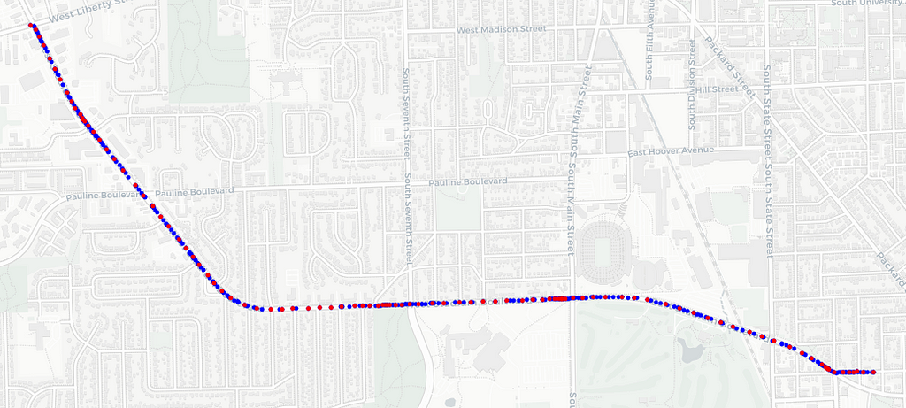
Modern cars, vans, and trucks are moving generators of telematics data. Vehicle telematics data streams usually carry various signals, the GPS location being one of the most frequent. You can also find signals such as instantaneous speed, acceleration, fuel tank or battery capacity, and other exotic signals like windshield-wiper status and external temperature.

GPS receivers typically sample data once per second (1 Hz), which is appropriate for most applications, but other vehicle sensors may have different signal generation frequencies. The signal generation frequency is programmable and generally balances telecommunications costs and the information content’s usefulness. Some signals are sent as they change, while others might get sent only after a given percent change to avoid unnecessary costs.

The telematics data streams have different approaches to packaging the signal values when sending them over the wireless connection. The most basic signal packaging approach independently sends each signal whenever it is generated or significantly changed. Each data packet contains the source identification, signal identification, and signal value. Another approach is to package all signal values as a standard record whenever each value changes. There is no preset emission frequency, and the unchanged values repeat on consecutive messages. We usually find this signal packaging approach on the receiving end of the communications link and when the sender uses the former approach.

The final approach, similar to the previous one, fixes the emission frequency, usually synchronized with the GPS, highlighting the importance of this signal in the process.

The second approach, which is the subject of this article, has some side effects, namely, the repetition of the GPS coordinates on all intermediate data packets between changes in the GPS signal. The following picture illustrates this effect on the Extended Vehicle Energy Dataset (EVED).

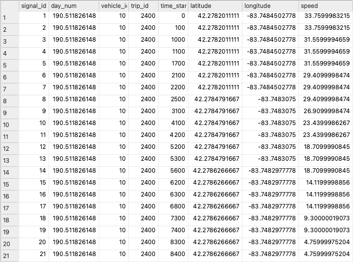
It is usual to handle data, as depicted in Figure 1, using the latitude and longitude as keys when removing duplicate rows. This technique keeps an aggregate of all the other columns, typically the first-row value. However, it may drastically reduce the number of rows in the dataset, rendering the data less valuable, similar to the third packaging approach.

Between changes in the GPS signal (rows 1, 8, and 14), all other records carry the original GPS coordinates, even if the vehicle is moving, as demonstrated by the speed signal in Figure 1 above. We can interpolate the geographic locations of the interim records, increasing the resolution of the GPS sensor and improving the dataset quality.

This article illustrates how to perform the GPS location interpolation mentioned above using map information and the speed signal.

Interpolation

GPS interpolation is the process of inferring geospatial locations missing from our input dataset using auxiliary data. If you like, this is akin to dead reckoning, a process through which GPS receivers infer the current location when you drive through a tunnel. Here, we apply a similar concept to a dataset where vehicle signals have higher sampling rates than the GPS receiver.

Dead reckoning uses a map to determine the road ahead and assumes a constant speed throughout the tunnel (or GPS blind spot). Here, we will use a similar approach. Knowing the map geometry between two consecutive and distinct GPS samples provides accurate distance information. If available, the speed signal helps us determine the approximate GPS location of the interim signals using simple kinematic calculations. Otherwise, we can assume a constant average speed between two consecutive locations. Fortunately, the EVED reports instantaneous speeds.

The first problem we must solve is measuring the distance between two consecutive and distinct GPS locations. We do this by using map information. We must use the map to avoid the error of measuring the geographical distance (as the crow flies) between the locations, as illustrated in Figure 2 below.

The GPS interpolation process requires auxiliary techniques to implement, such as map matching, map alignment, speed integration, and map projection. Let’s examine each one.

Map Matching

Map matching projects sequences of sampled GPS locations to the most likely trajectory over a digital map. I have already discussed this process in two other articles, exploring its applications to trajectory and speed predictions. Please review these two articles and their supporting code as they support this material.

After running the map-matching process, we collect the projection of the original GPS samples to the map edges and the sequence of map vertexes corresponding to the traveled route. Figure 2 above illustrates this, with the map vertexes in blue and the GPS projections in red. Before proceeding, we must compute the merged sequence of vertexes and GPS projections in a process that I call “map alignment.”

Map Alignment

As previously stated, the map-matching process produces two disjoint sets of points, namely the edge-projected GPS locations and the map vertexes, sequenced along the route direction. Before further processing, we must merge these location sets to ensure the correct sequencing between the sets. Unfortunately, the edge-projected GPS locations do not carry the edge information, so we must find the corresponding edge identified by the endpoint vertexes. This process produces a list of map edges with the matching GPS location projections.

Once done, we finish the map alignment process by converting the list of map edges to a complementary format: a list of GPS segments. We identify each GPS segment with its starting and ending locations and any map vertexes between them. Figure 3 below illustrates these concepts, with the blue bar identifying the map edge and the red bar identifying the GPS segment.

Now, we can examine and process each GPS segment separately. To better illustrate this concept, the first GPS segment of Figure 1 above would encompass rows one to eight along any map vertexes detected between them.

The typical GPS segment illustrated in Figure 3 above would have a set of signal records corresponding to each endpoint. Figure 1 shows that the first two GPS locations have seven and six records, respectively. We aim to project those to the segment’s geography using whatever information we can collect about the car’s motion. Fortunately, the EVED has both the timestamps and the recorded vehicle speed. We can reconstruct the displacements along the segment with some kinematics and place the interpolated GPS locations.

If you have ever studied kinematics, you know that:

On a velocity-time graph, the area under the curve is the change in position.

To recover the estimated distances between consecutive projected GPS locations, we need to compute the integral of the time versus speed.

Speed Integration

Figure 1 above shows that, for each record, we have values for the timestamp, measured in milliseconds since the trip started, and the car velocity, measured in kilometers per hour. To reconstruct all the intermediary distances, we compute a simple trapezoidal integral for each step and then adjust for the actual GPS segment length computed along the map.

The final adjustment step is needed because the speed signal will have some noise, which is assumed to have the same distribution throughout. Therefore, the distance computed from the integral will generally differ from the map distance.

To bridge this difference, we compute a correction factor between both distances, which allows us to calculate the adjusted distances between projected GPS locations. With this final information, we can now interpolate the repeated GPS locations along the segment.

Map Projection

The final step of the interpolation process is transferring the extra and repeated GPS locations to the map geometry. We compute each position using the previous one and move in the segment’s direction according to the previously calculated distance. Figure 4 below illustrates this process.

To respect the map geometry, the algorithm must consider map vertices between successive GPS locations during computation. In the case depicted in Figure 4 above, the initial GPS location in red had four repetitions that we could project to the new green points using both the signal timestamps and the recorded speeds. The algorithm must correctly assign the distances even when crossing a map vertex, as depicted.

When projecting the interpolated GPS locations, the algorithm uses the segment heading, the previous location, and the interim distance to compute the next point using a well-known formula.

The final set of GPS locations, including the sampled and interpolated ones, is stored for later use. Let’s see how this is done.

Implementation

Before trying to run this article’s code, read the prerequisite articles and run their code. This article’s code requires you to download and generate a database containing the EVED data, which is already map-matched, and the projected link durations. Please see the reference materials below.

The Python code that implements the concepts described in this article is available in the accompanying GitHub repository. You must execute the main script from the command line to interpolate all trips.

uv run interpolate-gps.py

This script iterates through all trips and processes one at a time. The first step is to load the map-matched trip polyline, where each point is a map vertex (the blue dots in the previous figures). These polylines were generated in earlier articles and should be stored in the database as encoded strings.

Polyline Decoding

Decoding the polyline requires a dedicated function adapted from the public Valhalla repositories.

https://medium.com/media/c96e8d54319e66d6351e6bf0ab0204cf/href

GPS Segment Generation

Next, the script collects and aligns the map-matched trip data (the red dots) with the map vertexes. This processing results in a list of GPS segments, structures containing the sequential pairs of map-matched GPS locations with any map vertexes in between.

https://medium.com/media/6fa257bef2bf8e68f80aa1ba629314c6/href

We use a function that accepts a Pandas DataFrame containing the original trajectory with the unique locations and the map-matched trajectory polyline to compute the list of GPS segments.

https://medium.com/media/15d0a04d2db14867cc9566ee81ebf881/href

The code then computes the repeated location projections along the segment’s geometry for each GPS segment. Note that this only occurs for the repeated locations corresponding to the starting GPS point. The end GPS point is repeated as the starting point of the next segment in the sequence.

We use a dedicated trajectory class to help us calculate GPS segments. As you can see from Figure 7 above, the function initializes the trajectory object using the sequence of distinct GPS locations, the corresponding timestamps, and the database identifiers for each point. This object then merges itself with the decoded polyline to return a …

The dead reckoning function projects the repeated locations using the GPS segment, the calculated distances, and known durations.

https://medium.com/media/97acaa061aeb3e197631eff46a52cdf1/href

The function above generates a list of points containing all the projections from the first GPS location, annotated with the row identifiers for later database insertion. This way, the code that uses these projected locations can refer back to the original row of data.

https://medium.com/media/349e9a5ef85d4caaf455d2cedb03c76f/href

We use the function below to compute a location based on a source location, a bearing, and a distance. The bearing is the angle measured in degrees from true North in the clockwise direction, so the East is 90 degrees and the South is 180 degrees.

https://medium.com/media/c0f06015dddda9fd52ac7561a2ebd3c6/href

We can now see how the main function loop integrates all these components. It is worth noting that the code keeps two copies of the original map-matched trajectory, one with the whole data and the second with only the unique locations (see lines 11–14 below).

https://medium.com/media/82fcd2f31ec7b3440a0ba4370506cde5/href

The last thing the code does is insert the interpolated locations into the database in a dedicated table that is 1:1 related to the original signals table.

https://medium.com/media/75d2418cdf7fa51d9abc99d3f6419d12/href

The refined data can now be used for an interesting case study, identifying road sections subject to the harshest braking and acceleration.

Case Study: Harsh Braking

With the added resolution of the interpolated GPS locations, we can gain better insights into vehicle behavior and make more precise computations. To illustrate how to use the improved location resolution, we study where cars break the harshest by computing an interesting movement feature: the jerk (or jolt). We can reliably compute this kinematic entity with shorter time intervals and corresponding speeds.

The zones of the harshest braking can be highlighted on a map using the derived interpolated GPS locations to calculate the instantaneous jerk through the third derivative of the r(t) function, where r is the displacement and t is time.

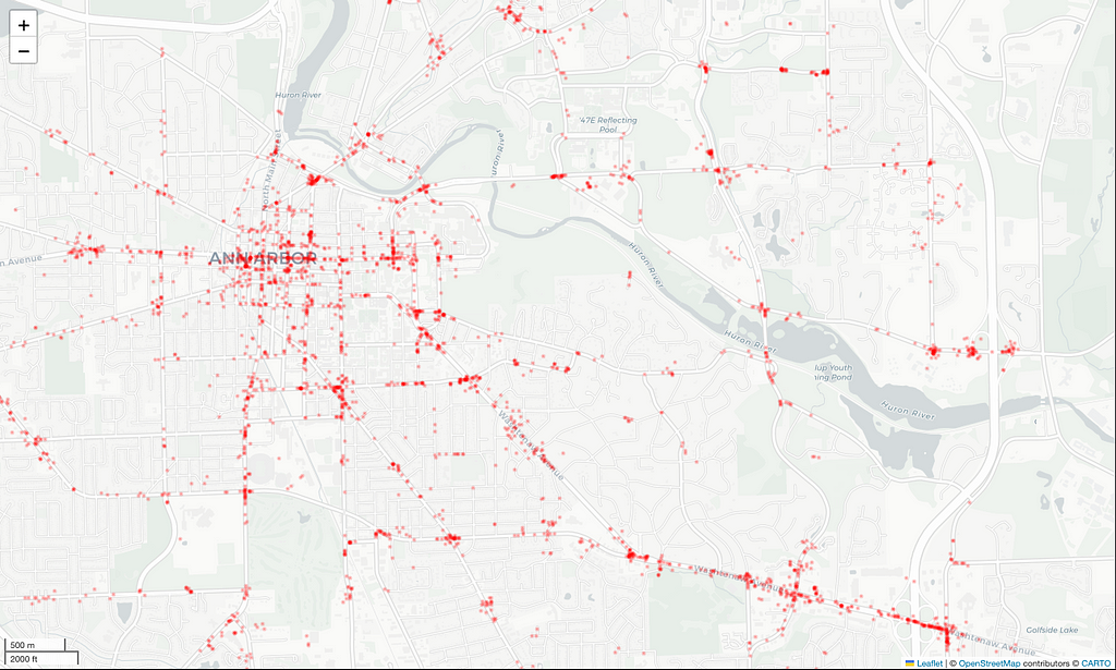
Figure 14 below shows the results of plotting the harshest brakes computed as values lower than 𝜇-3𝜎 of the jerk distribution. You can interact with this map through a dedicated Jupyter notebook.

Conclusion

In this article, we have looked at the problem of interpolating GPS locations using maps and intermediate signals, such as time and speed. After map-matching the sampled GPS locations, we retrieved the corresponding ma-generated tree containing the inferred trajectory path, and we used those geometries to project the missing GPS locations to the “correct” places using the known speeds and interim durations. After interpolating all EVED data, we used it to detect the areas in Ann Harbor where we expect to see the harshest braking as a proxy for possibly hazardous spots.

Credits

I used Grammarly to review the writing and accepted several of its rewriting suggestions.

JetBrains’ AI assistant wrote some of the code, and it has become a staple of my everyday work with Python.

Reference

• Map-Matching for Trajectory Prediction
• Map-Matching for Speed Prediction

Graphs of Motion — The Physics Hypertextbook

Movable Type Scripts — Calculate distance, bearing, and more between Latitude/Longitude points

João Paulo Figueira is a Data Scientist at tb.lx by Daimler Truck in Lisbon, Portugal.

---

GPS Interpolation Using Maps and Kinematics was originally published in Towards Data Science on Medium, where people are continuing the conversation by highlighting and responding to this story.

​How do you apply dead reckoning to your geospatial dataset?The picture above illustrates the GPS interpolation process. The red dots represent the known and repeated GPS locations, with more than one location per dot, while the blue dots represent the inferred locations of the repeated points along the road using the vehicle’s speed. (Image created by the author using OpenStreetMap data and imagery.)Modern cars, vans, and trucks are moving generators of telematics data. Vehicle telematics data streams usually carry various signals, the GPS location being one of the most frequent. You can also find signals such as instantaneous speed, acceleration, fuel tank or battery capacity, and other exotic signals like windshield-wiper status and external temperature.GPS receivers typically sample data once per second (1 Hz), which is appropriate for most applications, but other vehicle sensors may have different signal generation frequencies. The signal generation frequency is programmable and generally balances telecommunications costs and the information content’s usefulness. Some signals are sent as they change, while others might get sent only after a given percent change to avoid unnecessary costs.The telematics data streams have different approaches to packaging the signal values when sending them over the wireless connection. The most basic signal packaging approach independently sends each signal whenever it is generated or significantly changed. Each data packet contains the source identification, signal identification, and signal value. Another approach is to package all signal values as a standard record whenever each value changes. There is no preset emission frequency, and the unchanged values repeat on consecutive messages. We usually find this signal packaging approach on the receiving end of the communications link and when the sender uses the former approach.The final approach, similar to the previous one, fixes the emission frequency, usually synchronized with the GPS, highlighting the importance of this signal in the process.The second approach, which is the subject of this article, has some side effects, namely, the repetition of the GPS coordinates on all intermediate data packets between changes in the GPS signal. The following picture illustrates this effect on the Extended Vehicle Energy Dataset (EVED).Figure 1 — Data from the EVED shows how often the GPS location repeats while the vehicle moves. (Image source: Author)It is usual to handle data, as depicted in Figure 1, using the latitude and longitude as keys when removing duplicate rows. This technique keeps an aggregate of all the other columns, typically the first-row value. However, it may drastically reduce the number of rows in the dataset, rendering the data less valuable, similar to the third packaging approach.Between changes in the GPS signal (rows 1, 8, and 14), all other records carry the original GPS coordinates, even if the vehicle is moving, as demonstrated by the speed signal in Figure 1 above. We can interpolate the geographic locations of the interim records, increasing the resolution of the GPS sensor and improving the dataset quality.This article illustrates how to perform the GPS location interpolation mentioned above using map information and the speed signal.InterpolationGPS interpolation is the process of inferring geospatial locations missing from our input dataset using auxiliary data. If you like, this is akin to dead reckoning, a process through which GPS receivers infer the current location when you drive through a tunnel. Here, we apply a similar concept to a dataset where vehicle signals have higher sampling rates than the GPS receiver.Dead reckoning uses a map to determine the road ahead and assumes a constant speed throughout the tunnel (or GPS blind spot). Here, we will use a similar approach. Knowing the map geometry between two consecutive and distinct GPS samples provides accurate distance information. If available, the speed signal helps us determine the approximate GPS location of the interim signals using simple kinematic calculations. Otherwise, we can assume a constant average speed between two consecutive locations. Fortunately, the EVED reports instantaneous speeds.The first problem we must solve is measuring the distance between two consecutive and distinct GPS locations. We do this by using map information. We must use the map to avoid the error of measuring the geographical distance (as the crow flies) between the locations, as illustrated in Figure 2 below.Figure 2 — Blue dots are map vertexes, while red dots are map-matched GPS locations. The interpolated locations will occur along the blue line, and we must use the distance between consecutive samples along the red line’s geometry. The green line represents the distance between consecutive GPS locations without considering the map geometry, while the red line uses the map geometry. In this case, the red line is longer than the green one. (Image source: Author)The GPS interpolation process requires auxiliary techniques to implement, such as map matching, map alignment, speed integration, and map projection. Let’s examine each one.Map MatchingMap matching projects sequences of sampled GPS locations to the most likely trajectory over a digital map. I have already discussed this process in two other articles, exploring its applications to trajectory and speed predictions. Please review these two articles and their supporting code as they support this material.After running the map-matching process, we collect the projection of the original GPS samples to the map edges and the sequence of map vertexes corresponding to the traveled route. Figure 2 above illustrates this, with the map vertexes in blue and the GPS projections in red. Before proceeding, we must compute the merged sequence of vertexes and GPS projections in a process that I call “map alignment.”Map AlignmentAs previously stated, the map-matching process produces two disjoint sets of points, namely the edge-projected GPS locations and the map vertexes, sequenced along the route direction. Before further processing, we must merge these location sets to ensure the correct sequencing between the sets. Unfortunately, the edge-projected GPS locations do not carry the edge information, so we must find the corresponding edge identified by the endpoint vertexes. This process produces a list of map edges with the matching GPS location projections.Once done, we finish the map alignment process by converting the list of map edges to a complementary format: a list of GPS segments. We identify each GPS segment with its starting and ending locations and any map vertexes between them. Figure 3 below illustrates these concepts, with the blue bar identifying the map edge and the red bar identifying the GPS segment.Figure 3 — The map alignment process correctly sequences the map vertexes and the projected GPS locations and splits the resulting list into GPS segments, shown in red. Note that each GPS segment contains the projected GPS endpoints and all the included map vertexes within. (Image source: Author)Now, we can examine and process each GPS segment separately. To better illustrate this concept, the first GPS segment of Figure 1 above would encompass rows one to eight along any map vertexes detected between them.The typical GPS segment illustrated in Figure 3 above would have a set of signal records corresponding to each endpoint. Figure 1 shows that the first two GPS locations have seven and six records, respectively. We aim to project those to the segment’s geography using whatever information we can collect about the car’s motion. Fortunately, the EVED has both the timestamps and the recorded vehicle speed. We can reconstruct the displacements along the segment with some kinematics and place the interpolated GPS locations.If you have ever studied kinematics, you know that:On a velocity-time graph, the area under the curve is the change in position.To recover the estimated distances between consecutive projected GPS locations, we need to compute the integral of the time versus speed.Speed IntegrationFigure 1 above shows that, for each record, we have values for the timestamp, measured in milliseconds since the trip started, and the car velocity, measured in kilometers per hour. To reconstruct all the intermediary distances, we compute a simple trapezoidal integral for each step and then adjust for the actual GPS segment length computed along the map.The final adjustment step is needed because the speed signal will have some noise, which is assumed to have the same distribution throughout. Therefore, the distance computed from the integral will generally differ from the map distance.To bridge this difference, we compute a correction factor between both distances, which allows us to calculate the adjusted distances between projected GPS locations. With this final information, we can now interpolate the repeated GPS locations along the segment.Map ProjectionThe final step of the interpolation process is transferring the extra and repeated GPS locations to the map geometry. We compute each position using the previous one and move in the segment’s direction according to the previously calculated distance. Figure 4 below illustrates this process.Figure 4 — The map projection process uses the integrated distances and the GPS segment headings to calculate where to place the projected locations. From left to right, we use the position of the original GPS locations in red or the map vertexes in blue and the corresponding heading and distance to calculate the projected green GPS location. (Image source: Author)To respect the map geometry, the algorithm must consider map vertices between successive GPS locations during computation. In the case depicted in Figure 4 above, the initial GPS location in red had four repetitions that we could project to the new green points using both the signal timestamps and the recorded speeds. The algorithm must correctly assign the distances even when crossing a map vertex, as depicted.When projecting the interpolated GPS locations, the algorithm uses the segment heading, the previous location, and the interim distance to compute the next point using a well-known formula.The final set of GPS locations, including the sampled and interpolated ones, is stored for later use. Let’s see how this is done.ImplementationBefore trying to run this article’s code, read the prerequisite articles and run their code. This article’s code requires you to download and generate a database containing the EVED data, which is already map-matched, and the projected link durations. Please see the reference materials below.The Python code that implements the concepts described in this article is available in the accompanying GitHub repository. You must execute the main script from the command line to interpolate all trips.uv run interpolate-gps.pyThis script iterates through all trips and processes one at a time. The first step is to load the map-matched trip polyline, where each point is a map vertex (the blue dots in the previous figures). These polylines were generated in earlier articles and should be stored in the database as encoded strings.Polyline DecodingDecoding the polyline requires a dedicated function adapted from the public Valhalla repositories.https://medium.com/media/c96e8d54319e66d6351e6bf0ab0204cf/hrefGPS Segment GenerationNext, the script collects and aligns the map-matched trip data (the red dots) with the map vertexes. This processing results in a list of GPS segments, structures containing the sequential pairs of map-matched GPS locations with any map vertexes in between.https://medium.com/media/6fa257bef2bf8e68f80aa1ba629314c6/hrefWe use a function that accepts a Pandas DataFrame containing the original trajectory with the unique locations and the map-matched trajectory polyline to compute the list of GPS segments.https://medium.com/media/15d0a04d2db14867cc9566ee81ebf881/hrefThe code then computes the repeated location projections along the segment’s geometry for each GPS segment. Note that this only occurs for the repeated locations corresponding to the starting GPS point. The end GPS point is repeated as the starting point of the next segment in the sequence.We use a dedicated trajectory class to help us calculate GPS segments. As you can see from Figure 7 above, the function initializes the trajectory object using the sequence of distinct GPS locations, the corresponding timestamps, and the database identifiers for each point. This object then merges itself with the decoded polyline to return a …The dead reckoning function projects the repeated locations using the GPS segment, the calculated distances, and known durations.https://medium.com/media/97acaa061aeb3e197631eff46a52cdf1/hrefThe function above generates a list of points containing all the projections from the first GPS location, annotated with the row identifiers for later database insertion. This way, the code that uses these projected locations can refer back to the original row of data.https://medium.com/media/349e9a5ef85d4caaf455d2cedb03c76f/hrefWe use the function below to compute a location based on a source location, a bearing, and a distance. The bearing is the angle measured in degrees from true North in the clockwise direction, so the East is 90 degrees and the South is 180 degrees.https://medium.com/media/c0f06015dddda9fd52ac7561a2ebd3c6/hrefWe can now see how the main function loop integrates all these components. It is worth noting that the code keeps two copies of the original map-matched trajectory, one with the whole data and the second with only the unique locations (see lines 11–14 below).https://medium.com/media/82fcd2f31ec7b3440a0ba4370506cde5/hrefThe last thing the code does is insert the interpolated locations into the database in a dedicated table that is 1:1 related to the original signals table.https://medium.com/media/75d2418cdf7fa51d9abc99d3f6419d12/hrefThe refined data can now be used for an interesting case study, identifying road sections subject to the harshest braking and acceleration.Case Study: Harsh BrakingWith the added resolution of the interpolated GPS locations, we can gain better insights into vehicle behavior and make more precise computations. To illustrate how to use the improved location resolution, we study where cars break the harshest by computing an interesting movement feature: the jerk (or jolt). We can reliably compute this kinematic entity with shorter time intervals and corresponding speeds.Figure 13 — The jerk or jolt is the first derivative of the instantaneous acceleration. A high positive value means a sharp acceleration, while a significant negative value indicates a harsh brake. (Image source: Author using Wikipedia’s notation)The zones of the harshest braking can be highlighted on a map using the derived interpolated GPS locations to calculate the instantaneous jerk through the third derivative of the r(t) function, where r is the displacement and t is time.Figure 14 below shows the results of plotting the harshest brakes computed as values lower than 𝜇-3𝜎 of the jerk distribution. You can interact with this map through a dedicated Jupyter notebook.Figure 14 — The map above displays a portion of Ann Arbor’s map, with each red dot representing a point where the database recorded an exceptionally harsh brake. (Image created by the author using OpenStreetMap data and imagery.)ConclusionIn this article, we have looked at the problem of interpolating GPS locations using maps and intermediate signals, such as time and speed. After map-matching the sampled GPS locations, we retrieved the corresponding ma-generated tree containing the inferred trajectory path, and we used those geometries to project the missing GPS locations to the “correct” places using the known speeds and interim durations. After interpolating all EVED data, we used it to detect the areas in Ann Harbor where we expect to see the harshest braking as a proxy for possibly hazardous spots.CreditsI used Grammarly to review the writing and accepted several of its rewriting suggestions.JetBrains’ AI assistant wrote some of the code, and it has become a staple of my everyday work with Python.ReferenceMap-Matching for Trajectory PredictionMap-Matching for Speed PredictionGraphs of Motion — The Physics HypertextbookMovable Type Scripts — Calculate distance, bearing, and more between Latitude/Longitude pointsJoão Paulo Figueira is a Data Scientist at tb.lx by Daimler Truck in Lisbon, Portugal.GPS Interpolation Using Maps and Kinematics was originally published in Towards Data Science on Medium, where people are continuing the conversation by highlighting and responding to this story.  telematics, geospatial, hands-on-tutorials, gps, mapping Towards Data Science – MediumRead More

Add to favorites