5 practical use cases that prove Power Query is worth exploring.
I have a confession to make: I’ve been living under a rock 🪨. Not literally, but how else can I explain not discovering Power Query in Excel until now?
Imagine realising that all those hours spent wrangling VLOOKUPs, nesting IFs, and battling messy data could’ve been replaced with a few simple clicks.
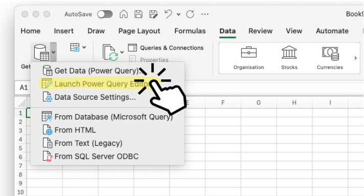
Power Query does everything Excel formulas could do — only faster, smarter, and way less frustrating. From merging datasets to effortless transformations and creating calculated columns, the possibilities are endless.
There are already tons of articles and videos out there with step-by-step guides to help you get started, so I won’t write another how-to. Instead, I’ll share the features that completely blew my mind with 5 use cases — and hopefully inspire you to dive in and explore this powerful tool yourself. 🚀
To demonstrate the remarkable functionality, I will use a simple e-commerce dataset consisting of two CSV files: one with customer data and the other with transaction data.
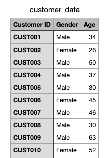
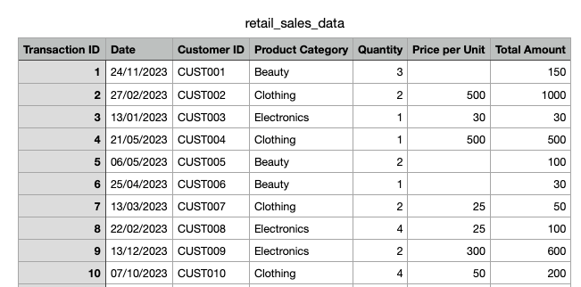
Use Case 1: Merging Datasets (A Smarter Alternative to VLOOKUP)
When it comes to combining data, we all turn to VLOOKUP. But let’s face it — VLOOKUP has its limitations.
Why Power Query is better than VLOOKUP✨:
- You can join data from multiple columns in one step (no need for repeated lookups).
- Your lookup column doesn’t have to be on the left — it works no matter where it’s located.
- It supports different join types (left, right, full, inner, anti), giving you more control over how data is combined.
- Unlike VLOOKUP, Power Query doesn’t limit you to joining on just one column.
- You can even handle messy datasets with typos using fuzzy matching!
How to merge datasets in Power Query 🔗:
- While on the Home tab select “Merge Queries”.
- Choose the two datasets (or files) you want to combine.
- Select the column to join on and specify the type of join (e.g., left join to keep all rows from one table, or inner join to match only overlapping rows).
- Once merged, select the columns you want to include in your final dataset.
- Load the transformed data back into Excel.
Done in seconds! ⏱️
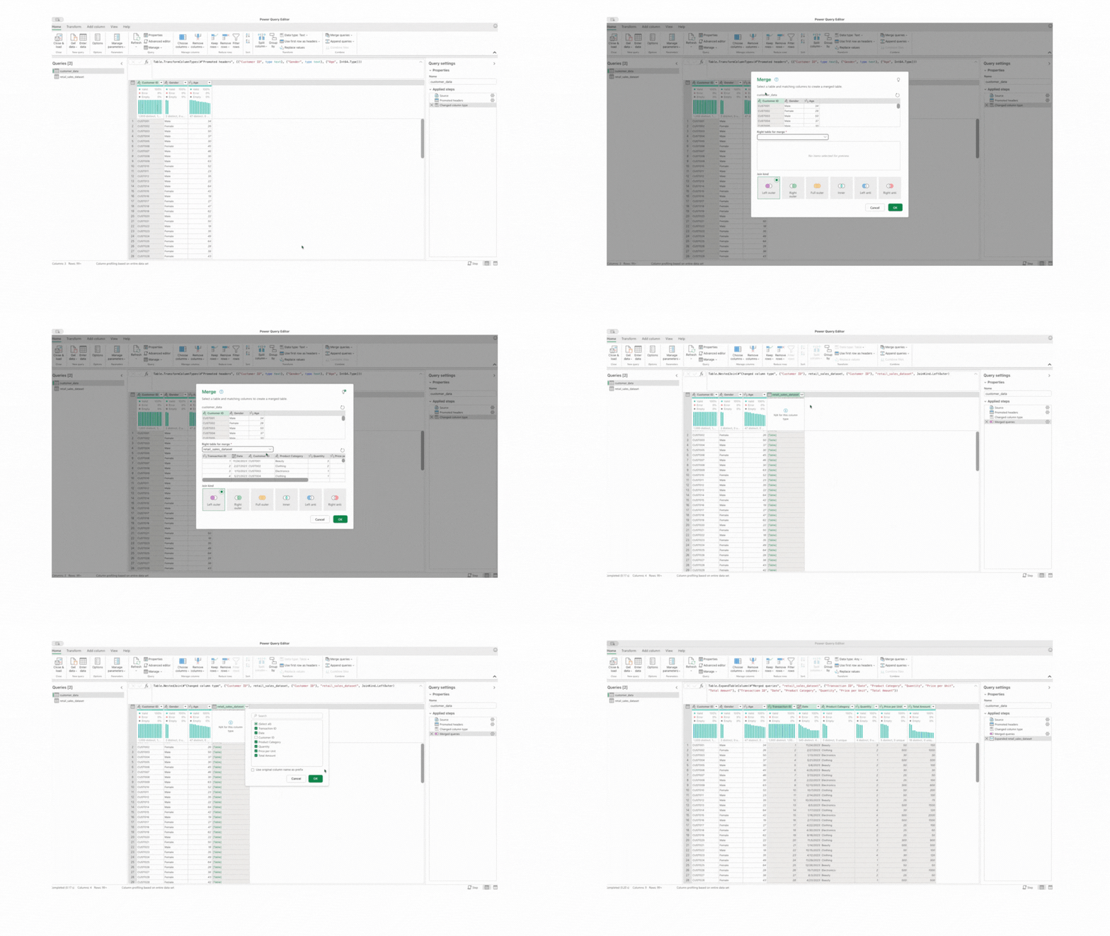
Use Case 2: Column Transformations
Power Query makes it super easy to transform your data. From quick calculations to date handling and creating bins, it does in seconds what could take minutes (or more) in Excel.
Let me show you how with a few examples. 👀
Perform Quick Calculations ➕➖➗✖️
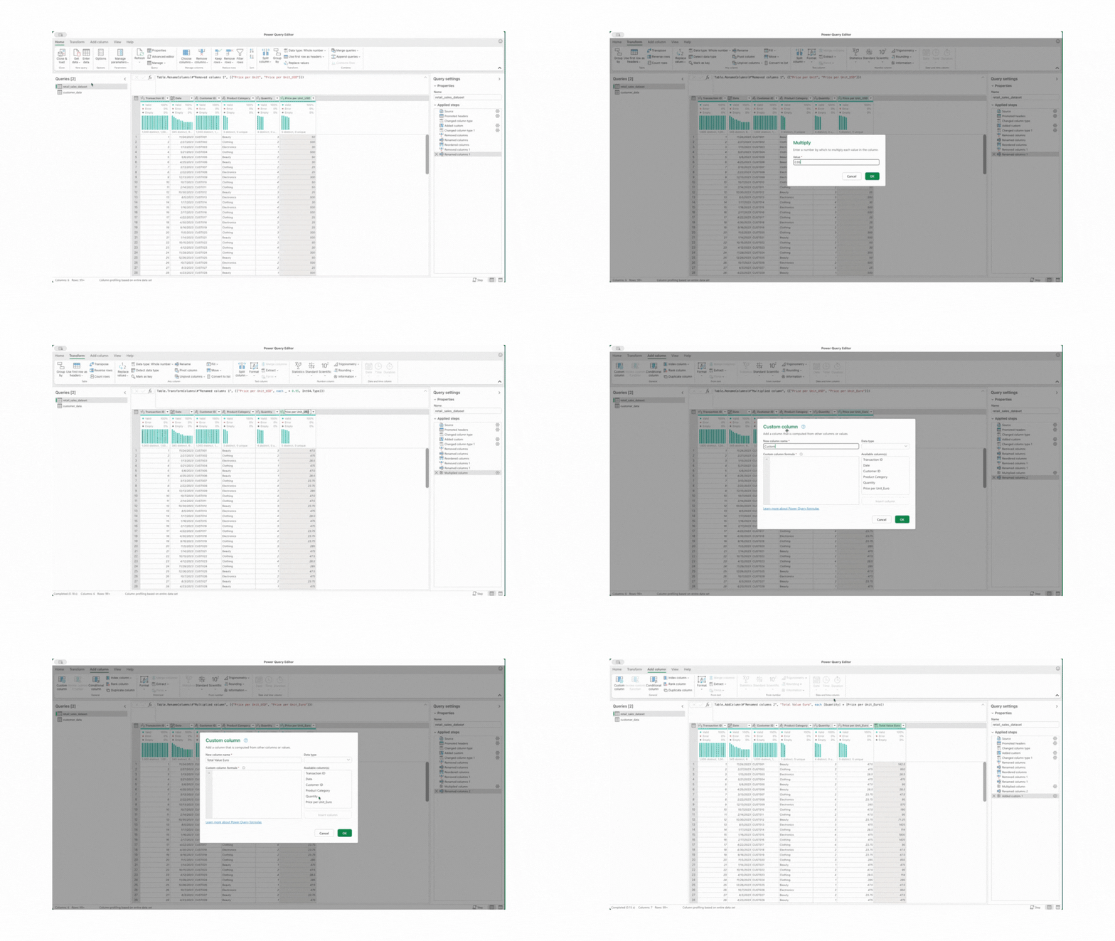
Let’s say you need to convert prices from USD to Euro and calculate the total value of your sales. In Power Query, you can:
- Go to the “Transform” tab and, under “Standard”, select “Multiply.”
- Multiply all the prices by 0.95 to convert the currencies.
- Add a new column to calculate total sales by multiplying the price by the quantity. To do this, go to the “Add Column” tab and select “Custom Column.”
All of this happens in just a few clicks.
Modify Dates with Ease 📅
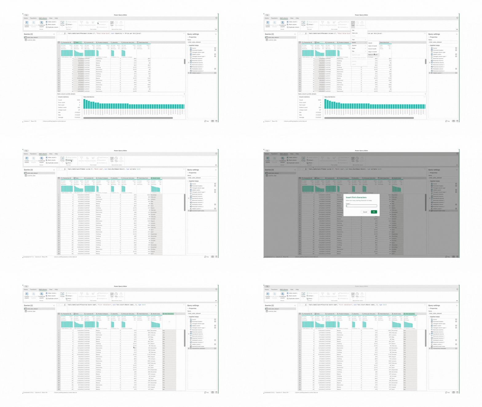
Power Query makes working with dates straightforward too. You can quickly extract the month name or display only the first three letters (e.g., Jan, Feb, Mar) for a cleaner look using built-in functionality.
- Select the column that is in Date format.
- Go to the “Add Column” tab, and under “Date”, select “Month” followed by “Name of the Month”.
- Select the new column that contains the name of the month. Under “Extract”, choose “First Characters”, and in the pop-up window, specify how many characters you want to extract (3 in this case).
No complicated formulas needed!
Create Bins Without Complex Formulas 📥
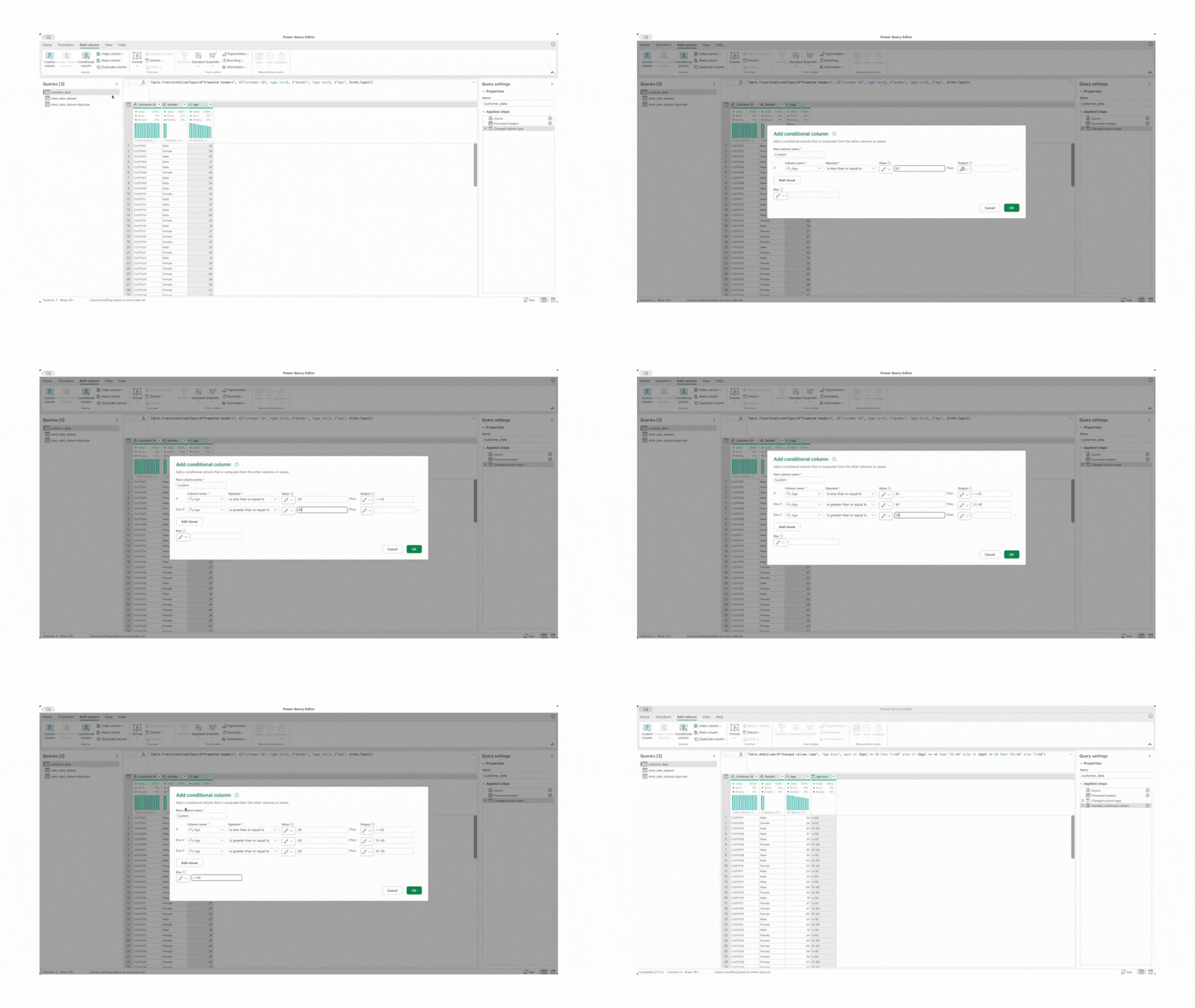
I don’t know about you, but I always forget the IF formula syntax for creating bins in Excel, and it can get pretty long if you have multiple ranges. But with Power Query, it’s much easier.
- If you’re using Windows, you’ve got the “Columns from Examples” feature. All you need to do is type one example of the bin range (e.g., “41–50”), and Power Query will automatically fill in the rest for you, saving you time.
- For those of us on Mac (like me), unfortunately, this feature isn’t available. But don’t worry, there’s a workaround! You can still create bins using the “Conditional Column” feature by setting logic rules to categorize your data into ranges.
Use Case 3: Filling in Missing Data 🔎
We’ve all worked with datasets with missing values — whether it is because of incomplete entries or data discrepancies. In most cases, you don’t want to leave this gaps, instead you want to fill them in. This is where Power Query becomes particularly useful.
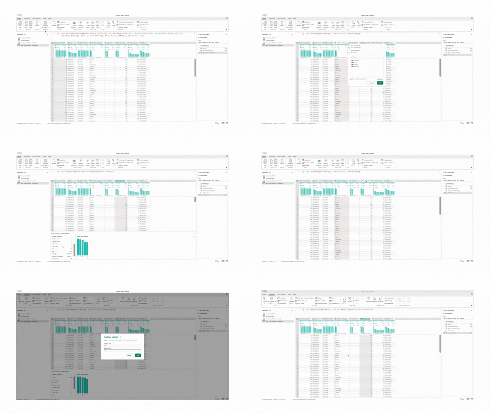
Let’s say we have missing values in the “Price per Unit” column for the “Beauty” category, and we want to replace those missing values with the average price for that category. Here’s how you can do it in a few simple steps:
- Filter the “Product Category” column to show only “Beauty” entries.
- With the “Price per Unit” column selected, check the average price for the Beauty category in the statistics section at the bottom of the screen.
- Remove the filter on the “Product Category” column to show all categories again.
- Select the “Price per Unit” column again, go to the “Transform” tab, and click on “Replace Values”.
- In the dialog box, enter “null” for the value you want to replace and the average price for the Beauty category in the “Replace With” field.
And just like that, you’ve filled in the missing data with the average value — all in a few clicks.
Use Case 4: Transforming Data for Better Analysis 🛠️
Power Query is great for transforming your data into a format to match the needs of your analysis.
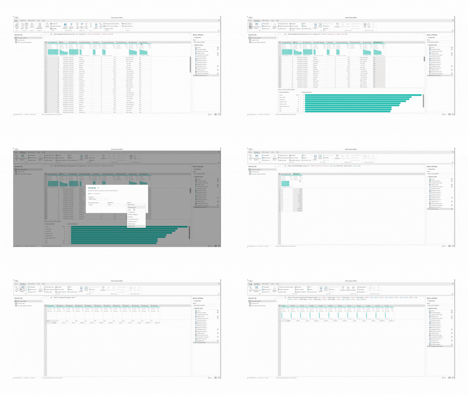
For example, if you want to summarise total sales per month and see the trend over time. You can use the “Group By” and “Transpose” functions.
Here’s how to do it in just 4 steps:
- Select the “Month” column to group your data by month.
- In the Transform tab, click on “Group By”.
- Add a new aggregation for “Total Value Euro” and select Sum to calculate the total sales for each month.
- Finally, click on “Transpose” to switch rows and columns, turning months into column headers.
Once you’re done, load the data back into Excel and build your line chart to visualize the sales trends over time!
Use Case 5. Custom Columns with M Formula Language 🪄
M formula language lets you go beyond the typical Power Query transformations, allowing for more advanced calculations and logic. It’s perfect when you need to create custom solutions for your data.
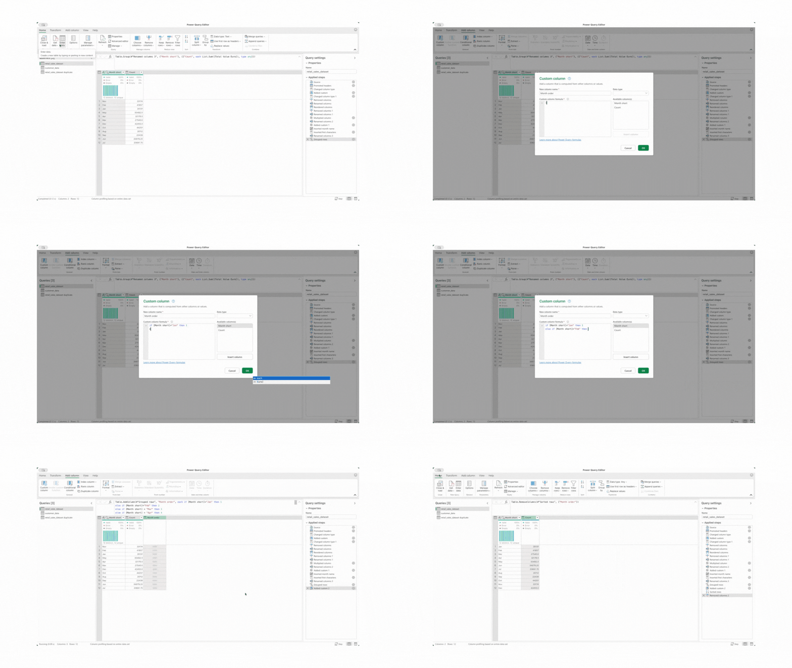
For example, let’s say the months in your sales data aren’t sorted correctly. Instead of manually rearranging them, you can use M formulas to assign a numerical value to each month, then sort them in the right order.
- Go to “Transform” and select “Custom column” option.
- In the pop up window type the logic using “if-else if” logic to assign a numerical value to each month.
- Sort by the new column in ASC order.
- You can even remove the “Month Order” column once the sorting is done.
After doing that, your months will be in the right order. 🏆🏆🏆
if [Month short] = "Jan" then 1
else if [Month short] = "Feb" then 2
else if [Month short] = "Mar" then 3
else if [Month short] = "Apr" then 4
else if [Month short] = "May" then 5
else if [Month short] = "Jun" then 6
else if [Month short] = "Jul" then 7
else if [Month short] = "Aug" then 8
else if [Month short] = "Sep" then 9
else if [Month short] = "Oct" then 10
else if [Month short] = "Nov" then 11
else if [Month short] = "Dec" then 12
else null
Last but not the least…
Power Query keeps track of every change in an applied steps log 💾, so if you want to go back and modify/undo anything, it’s super easy.
Feeling inspired? 🧙♂️
I hope you’re now as excited to try these features as I was! If I were you, I’d be jumping into Power Query right away.
Think you Know Excel? Take Your Analytics Skills to the Next Level with Power Query! was originally published in Towards Data Science on Medium, where people are continuing the conversation by highlighting and responding to this story.
5 practical use cases that prove Power Query is worth exploring.I have a confession to make: I’ve been living under a rock 🪨. Not literally, but how else can I explain not discovering Power Query in Excel until now?Imagine realising that all those hours spent wrangling VLOOKUPs, nesting IFs, and battling messy data could’ve been replaced with a few simple clicks.Image generated by the authorPower Query does everything Excel formulas could do — only faster, smarter, and way less frustrating. From merging datasets to effortless transformations and creating calculated columns, the possibilities are endless.There are already tons of articles and videos out there with step-by-step guides to help you get started, so I won’t write another how-to. Instead, I’ll share the features that completely blew my mind with 5 use cases — and hopefully inspire you to dive in and explore this powerful tool yourself. 🚀To demonstrate the remarkable functionality, I will use a simple e-commerce dataset consisting of two CSV files: one with customer data and the other with transaction data.These screens display samples of the first 10 rows from each CSV file (generated by the author)Use Case 1: Merging Datasets (A Smarter Alternative to VLOOKUP)When it comes to combining data, we all turn to VLOOKUP. But let’s face it — VLOOKUP has its limitations.Why Power Query is better than VLOOKUP✨:You can join data from multiple columns in one step (no need for repeated lookups).Your lookup column doesn’t have to be on the left — it works no matter where it’s located.It supports different join types (left, right, full, inner, anti), giving you more control over how data is combined.Unlike VLOOKUP, Power Query doesn’t limit you to joining on just one column.You can even handle messy datasets with typos using fuzzy matching!How to merge datasets in Power Query 🔗:While on the Home tab select “Merge Queries”.Choose the two datasets (or files) you want to combine.Select the column to join on and specify the type of join (e.g., left join to keep all rows from one table, or inner join to match only overlapping rows).Once merged, select the columns you want to include in your final dataset.Load the transformed data back into Excel.Done in seconds! ⏱️This gif explains the process of merging two files using Power Query (generated by the author)Use Case 2: Column TransformationsPower Query makes it super easy to transform your data. From quick calculations to date handling and creating bins, it does in seconds what could take minutes (or more) in Excel.Let me show you how with a few examples. 👀Perform Quick Calculations ➕➖➗✖️Let’s say you need to convert prices from USD to Euro and calculate the total value of your sales. In Power Query, you can:Go to the “Transform” tab and, under “Standard”, select “Multiply.”Multiply all the prices by 0.95 to convert the currencies.Add a new column to calculate total sales by multiplying the price by the quantity. To do this, go to the “Add Column” tab and select “Custom Column.”All of this happens in just a few clicks.This gif explains the process of performing quick calculations using Power Query (generated by the author)Modify Dates with Ease 📅Power Query makes working with dates straightforward too. You can quickly extract the month name or display only the first three letters (e.g., Jan, Feb, Mar) for a cleaner look using built-in functionality.Select the column that is in Date format.Go to the “Add Column” tab, and under “Date”, select “Month” followed by “Name of the Month”.Select the new column that contains the name of the month. Under “Extract”, choose “First Characters”, and in the pop-up window, specify how many characters you want to extract (3 in this case).No complicated formulas needed!This gif explains the process of modifying dates using Power Query (generated by the author)Create Bins Without Complex Formulas 📥I don’t know about you, but I always forget the IF formula syntax for creating bins in Excel, and it can get pretty long if you have multiple ranges. But with Power Query, it’s much easier.If you’re using Windows, you’ve got the “Columns from Examples” feature. All you need to do is type one example of the bin range (e.g., “41–50”), and Power Query will automatically fill in the rest for you, saving you time.For those of us on Mac (like me), unfortunately, this feature isn’t available. But don’t worry, there’s a workaround! You can still create bins using the “Conditional Column” feature by setting logic rules to categorize your data into ranges.This gif explains the process of creating bins using the “Conditional Column” feature (generated by the author)Use Case 3: Filling in Missing Data 🔎We’ve all worked with datasets with missing values — whether it is because of incomplete entries or data discrepancies. In most cases, you don’t want to leave this gaps, instead you want to fill them in. This is where Power Query becomes particularly useful.Let’s say we have missing values in the “Price per Unit” column for the “Beauty” category, and we want to replace those missing values with the average price for that category. Here’s how you can do it in a few simple steps:Filter the “Product Category” column to show only “Beauty” entries.With the “Price per Unit” column selected, check the average price for the Beauty category in the statistics section at the bottom of the screen.Remove the filter on the “Product Category” column to show all categories again.Select the “Price per Unit” column again, go to the “Transform” tab, and click on “Replace Values”.In the dialog box, enter “null” for the value you want to replace and the average price for the Beauty category in the “Replace With” field.And just like that, you’ve filled in the missing data with the average value — all in a few clicks.This gif explains the process of filling the missing values using Power Query (generated by the author)Use Case 4: Transforming Data for Better Analysis 🛠️Power Query is great for transforming your data into a format to match the needs of your analysis.For example, if you want to summarise total sales per month and see the trend over time. You can use the “Group By” and “Transpose” functions.Here’s how to do it in just 4 steps:Select the “Month” column to group your data by month.In the Transform tab, click on “Group By”.Add a new aggregation for “Total Value Euro” and select Sum to calculate the total sales for each month.Finally, click on “Transpose” to switch rows and columns, turning months into column headers.Once you’re done, load the data back into Excel and build your line chart to visualize the sales trends over time!This gif explains the process of using Group By and Transpose functions (generated by the author)Use Case 5. Custom Columns with M Formula Language 🪄M formula language lets you go beyond the typical Power Query transformations, allowing for more advanced calculations and logic. It’s perfect when you need to create custom solutions for your data.For example, let’s say the months in your sales data aren’t sorted correctly. Instead of manually rearranging them, you can use M formulas to assign a numerical value to each month, then sort them in the right order.Go to “Transform” and select “Custom column” option.In the pop up window type the logic using “if-else if” logic to assign a numerical value to each month.Sort by the new column in ASC order.You can even remove the “Month Order” column once the sorting is done.After doing that, your months will be in the right order. 🏆🏆🏆if [Month short] = “Jan” then 1else if [Month short] = “Feb” then 2else if [Month short] = “Mar” then 3else if [Month short] = “Apr” then 4else if [Month short] = “May” then 5else if [Month short] = “Jun” then 6else if [Month short] = “Jul” then 7else if [Month short] = “Aug” then 8else if [Month short] = “Sep” then 9else if [Month short] = “Oct” then 10else if [Month short] = “Nov” then 11else if [Month short] = “Dec” then 12else nullThis gif explains the process of using M formula language in Power Query (generated by the author)Last but not the least…Power Query keeps track of every change in an applied steps log 💾, so if you want to go back and modify/undo anything, it’s super easy.Feeling inspired? 🧙♂️I hope you’re now as excited to try these features as I was! If I were you, I’d be jumping into Power Query right away.Think you Know Excel? Take Your Analytics Skills to the Next Level with Power Query! was originally published in Towards Data Science on Medium, where people are continuing the conversation by highlighting and responding to this story. data-analytics, power-query, data-analysis, excel, data-science Towards Data Science – MediumRead More

 Add to favorites



0 Comments