A visual tour from classical statistics to the nuances of deep learning
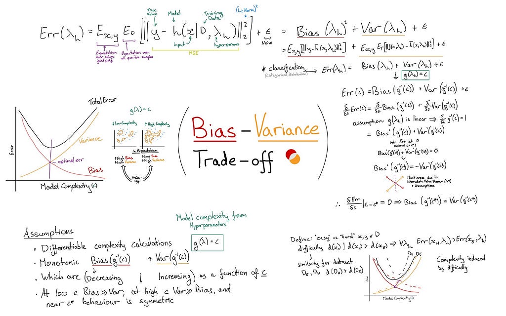
In deep learning the bias-variance trade-off is not straightforward and can often be the wrong thing to pay attention to. To understand why, we need to take a tour through inferential statistics, classical statistical learning methods, and machine learning robustness. We’ll end the article by touching on overparameterisation and the double descent phenomena.
Suggested background: Probability, Random Variables, Statistics, Linear Algebra, Calculus, Machine Learning, Deep Learning.
Bias and Variance in Inferential Statistics
Note: We are going to gloss some math in this section in favour of visual intuition. Given my focus on deep learning the particulars of inferential statistics would blow out the length of an already long article.
Imagine you travel back in time and take the place of a statistician in Allied Command during World War II. An intelligence officer tells you the following information:
- The Germans stamp sequential serial numbers on their tanks. So a tank with serial number 115 means it was the 115th tank produced. To date the Germans have produced an unknown number of tanks (N).
- When the allies destroy a tank we can find a serial number printed on it. The “destroyability” of a tank is independent of its serial number.
- We have a sample (size k) of serial numbers, X = (x₁, x₂, … xₖ).
- We need to use this sample to create an estimator N*.
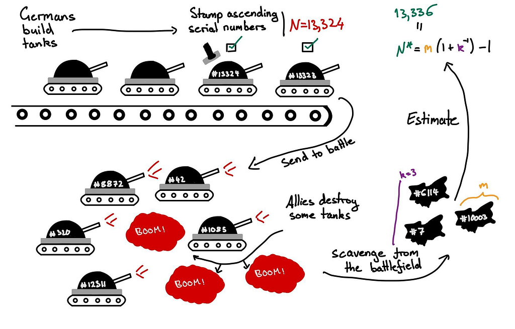
This is known as the German Tank Problem. In essence:
Given a manufacturing process which generates sequential serial numbers, how can you estimate the total production volume from a random sample?
Exploring an estimator
We’re going to start by looking at one possible estimator and explore its mathematical properties:

- N* is our estimator for N
- X is a random sample of size k
- m=max(X) is the largest serial number observed in the sample
We can use a Monte Carlo simulation to calculate the expected performance of N*:
- Draw N from a log-normal distribution (mean=200, large variance)
- Draw k from a Poisson distribution (λ=20)
- For 10,000 iterations, sample k values from [1..N] and compute N*
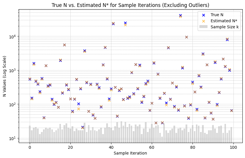
This simulates a range of possible worlds in which the sample data was collected. The plot below shows 100 iterations of the simulation for different values of N, k, and N*.
Unbiased estimator
We can see that the estimates are generally very accurate — sometimes over estimating the true value and sometimes underestimating it. We can plot the errors across all 10k iterations and see how they are distributed:
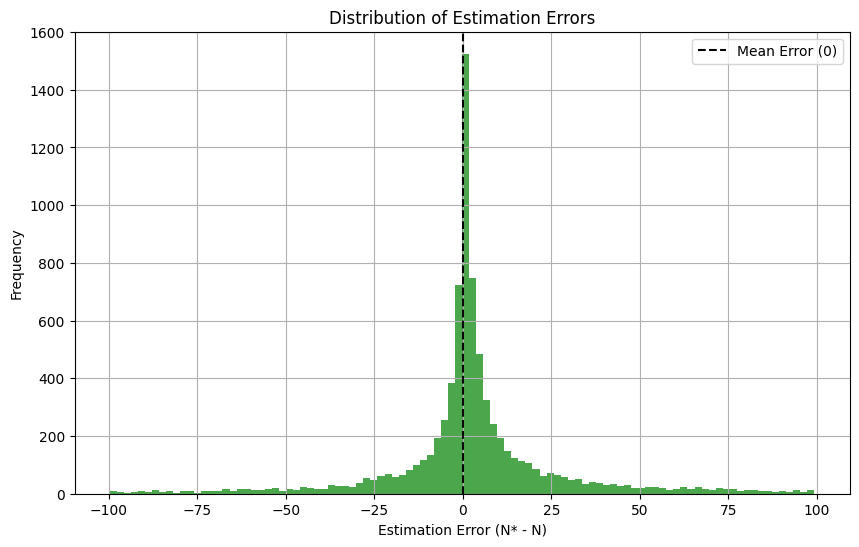
The plot shows that the mean error of N* is zero. That’s because this is a well known unbiased estimator. This means that on average errors cancel out, and N* approximates N in expectation. i.e. Averaged across all possible worlds.
Formally, the bias of an estimator of N is expressed as:
![text{Bias}(N^*)=N-mathbb{E}_{X|N,k}[N^*]](https://cdn-images-1.medium.com/max/374/1*57t_rrKUhNIATGRcr2GAJg.png)
The bias is the expected (signed) error of the estimator over all possible samples for a fixed N and k. If the expected error is 0 that means the estimator is unbiased. This is usually written as just the expectation over X rather than X|N,k. I’ve used extra subscripts just to emphasise a point.
Note that this is sometimes written as:
![text{Bias}(N^*)=mathbb{E}[N-mathbb{E}[N^*]]](https://cdn-images-1.medium.com/max/347/1*Uu3LEE1jvoCz9qTyUl4bIg.png)
In this situation we can show that the extra expectation is not necessary. N is an unknown but concrete value and the same is true of the expected value of N*. The expected value of a constant is just the constant so we can drop the extra notation.
Variance of an estimator
Variance quantifies how much the estimates will vary across different possible worlds. Our error plot shows estimates cluster around 0, with slight skew due to priors on N and k. If we look at the ratio k/N we can see how the estimator performs with larger and larger samples:
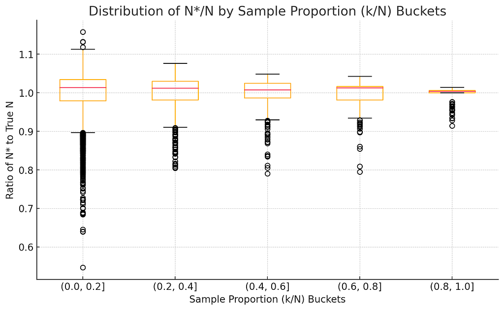
The intuitive result is that for an unbiased estimator, collecting a larger sample leads to more accurate results. The true variance of N* is:

The standard deviation (N/k) can be thought of as the average gap between elements in a random sample of size k. For example: if the true value is N=200 and the sample size is k=10, then the average gap between values in the sample is 20. Hence, we would expect most estimates to be in the range 200±40.
It can be shown that this is the minimum variance that can be achieved by any unbiased estimator. In frequentist statistics this is known as the Uniformly Minimum Variance Unbiased Estimator (UMVUE). Put another way: to achieve lower variance you need a biased estimator.
Formally, the variance of an estimator of N is expressed as:
![text{Var}(N^*)=mathbb{E}_{X|N,k}[(N^*-mathbb{E}_{X|N,k}[N^*])²]](https://cdn-images-1.medium.com/max/517/1*7zU8pVqUJBaNJ1_RJNGRbw.png)
Notice that the variance is the expectation around the estimated value rather than around the true value. If we had a biased estimator we would be evaluating the spread around that biased estimate.
Test your understanding: do you see why we need the expectation around the outer term? N* is a random variable and so we need an expectation over all possible X in order to get a concrete value for it.
Sufficient information
There’s something you may have noticed about our estimator: it seemingly throws away a lot of information in our sample. If our sample has k values why should our estimator use only 1 value?
First, some quick definitions:
- A “statistic” is a function of data (usually of a sample).
- A “sufficient statistic” is one that contains the maximal “information” about the population parameter we are trying to estimate.
It’s possible to show that there isn’t any extra information in the sample once we know the maximum and the sample size k. The reason concerns the likelihood function for values of N given a sample X.
The likelihood function
Consider all possible k-sized subsets of [1..N]. For any given sample the only possible values of N are in the range [max(X), ∞]. i.e. It’s not possible to get a sample containing max(X) if N<max(X). The probability of getting any one k-sized sample is based on how many ways there are of choosing a set of size k from N possible values. The likelihood function is shown below. Notice how the likelihood function for a fixed sample is only concerned with k and m=max(X).
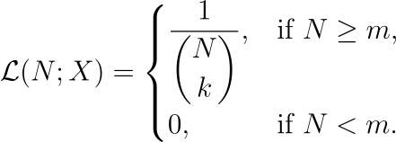
A likelihood function ℒ(θ;x) measures how probable an observation x is under different values of θ (e.g. N). We can use it to find a value of θ which maximises the probability of seeing x without telling us anything about the probability of θ itself.
Maximum likelihood
Suppose k=5 and m=60, then N ≥ 60. The maximum likelihood occurs at N=m=60. While most values of N are unlikely the likelihood function identifies N=60 as most likely for this sample.
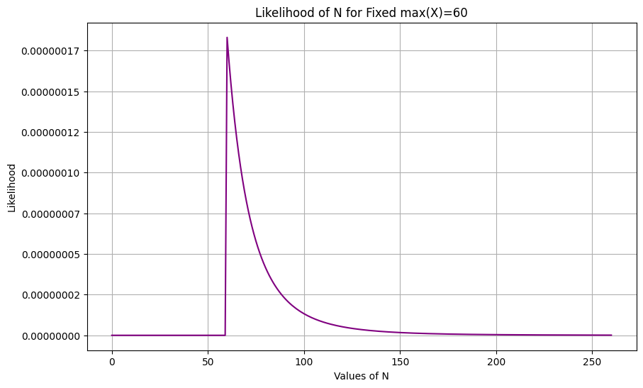
First, notice that all values of N are very unlikely. Then, remember that for a fixed value of (m, k) the likelihood function tells us the probability of seeing that value of m for each possible value of N. Just because m=60 is most probable at N=60 doesn’t make it a good estimate!
The most likely estimate is not necessarily the best one.
Fisher information
Fisher information quantifies sample informativeness. If many values of N are likely, information is low; if there’s a sharp likelihood peak around the true value then information is high. As a rough guide, Fisher information tells us how much we could possibly know about the true distribution from a random sample.
A sufficient statistic
A “sufficient statistic” contains all of the information about the parameter in question. I won’t go into the proof here but a statistic is sufficient if it is the Maximum Likelihood Estimator (MLE). If the MLE is biased we can use “bias correction” to produce a better estimate but we can’t find another statistic which provides more information.
An intuitive explanation
Not all sample data provides useful information. Specific to the German Tank Problem we can see that:
- The sample probability depends on k and max(X).
- Values of N near max(X) are more likely to produce samples which happen to contain max(X).
- All k-sized samples containing max(X) are equally probable.
- So the sample contains no more information about the true value of N beyond knowing k and max(X).
A biased estimator
Using max(X)=m as an estimator would almost always underestimate N as the probability of getting N in a sample is 1/(N choose k). On the other hand, if we did get a sample which contained N our original estimator N* could give a big overestimate. Suppose k=1 and our sample happened to contain N=1000. Then our estimate of N*=2m-1=1999 would be much too large.
It’s hopefully obvious that this is a terrible argument for using max(X) as our estimator for N. To check let’s compare the Mean Square Error (MSE) of the two estimators to see how they perform:
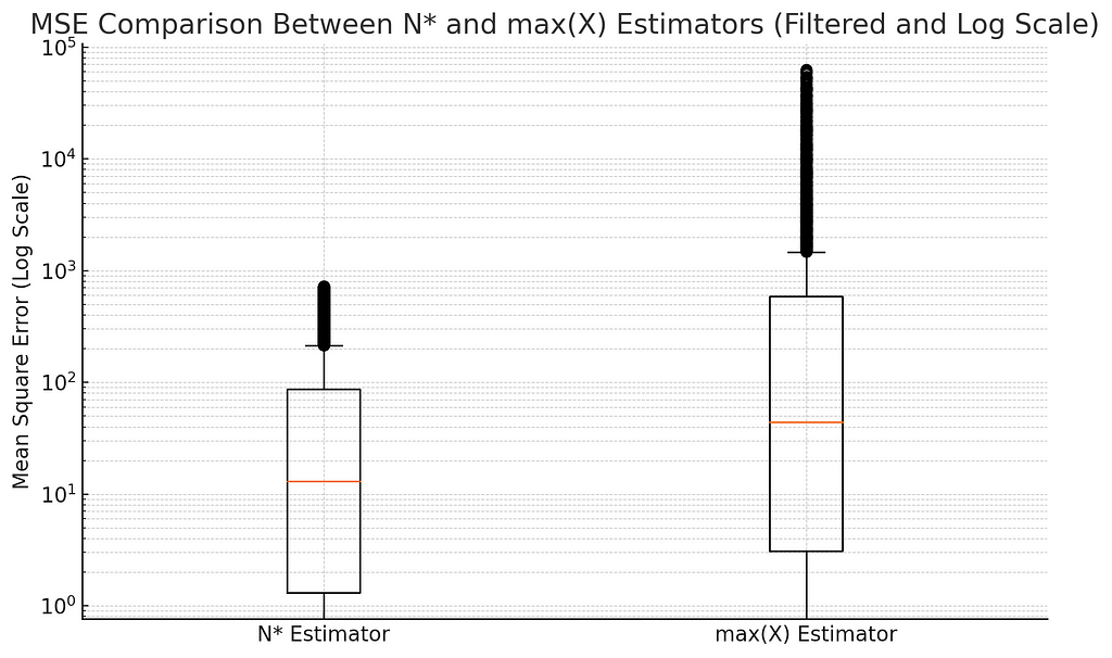
Notice how much worse the estimator max(X) is. Note that almost all of that error is attributed to its bias. If we plot the distribution of estimated values we can see that max(X) consistently produces estimates in a narrower range.
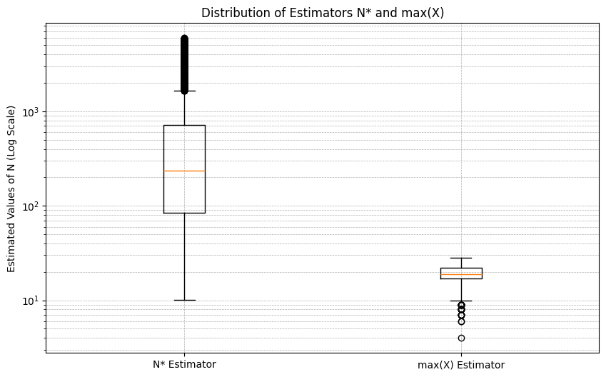
I’ll skip the proof and we’ll rely on the visualisation to see that max(X) has a significantly lower variance than N*. Just remember that the proper definition for estimator variance is the expected spread around the expected estimated value.
The bias-variance decomposition
By convention the total error we are trying to minimise is the mean square error (MSE). If you’re curious you can read this discussion about why we use MSE. I’ll leave off the subscripts this time but remember that we are calculating the expectation over all possible samples:
![text{Err}=mathbb{E}left[(N-N^*)²right]](https://cdn-images-1.medium.com/max/279/1*7jFUMoI91r8V5rY0Ogmr2w.png)
This this can be factored into a bias² term and a variance term. The derivation is useful to understand. We start by introducing -E[N*]+E[N*], then grouping terms, and expanding the quadratic:
![text{Err} &= E[(N — N^*)²] \ &= Eleft[left((N — E[N^*]) + (E[N^*] — N^*)right)²right] \ &= Eleft[(N — E[N^*])² + 2(N — E[N^*])(E[N^*] — N^*) + (E[N^*] — N^*)²right] \ &= E[(N — E[N^*])²] + 2E[(N — E[N^*])(E[N^*] — N^*)] + E[(E[N^*] — N^*)²] \ &= E[(N — E[N^*])²] + 0 + E[(E[N^*] — N^*)²] \ &= text{Bias}²(N^*) + text{Var}(N^*)](https://cdn-images-1.medium.com/max/1000/1*oVjMAG5dHH9_9IkOFb5tNA.png)
The biggest confusion may come at the second last line:
- The left term is bias² if we ignore the redundant expectation.
- The centre term comes to 0 after expanding and applying the expectation operator over the expanded terms.
- The right term is just variance depending on which term is subtracted before squaring the result.
A more general derivation can be found on the Wikipedia article on the bias-variance trade-off.
The total expected error is a combination of the error from the bias of our estimator and the variance. Here’s a subtle question: if the model is biased then shouldn’t a high variance allow it to sometimes get an accurate answer? Why would the total expected error be a sum of bias² and variance instead of some other function that takes this into account?
The decomposition above explains how it happens mathematically but perhaps not intuitively. For building intuition, consider the effect that squaring has on highly inaccurate estimates. Also consider that the bias² itself is not sufficient to account for all of the expected squared error.
An optimal estimator?
We’ve shown the expected error for our estimator. On average, given a random sample, how far off would our estimator be from the true value that generated that sample? An estimator that’s consistently off but predicts a narrower spread might be better than an estimator which is consistently on-point but has a much wider spread of predictions around that point.
Can we find a balance point in the German Tank Problem where we trade off bias and variance to make a better estimate? Ignoring a constant term (+ C) such a function would look like this:

This will sit somewhere between g(k)=1 and g(k)=(1+1/k). Can you work out why? Using 1 * m is the MLE which is biased but low variance. Using (1+1/k) is just N* without a constant. We know that N* is an unbiased estimator (UMVUE) with higher variance then m. So somewhere between the MLE and the UMVUE we could find the “optimal” estimator.
It turns out we can’t find an optimal function g(k) without knowing the true value of N, which is the number we are trying to estimate!
The Wikipedia page on the problem describes Bayesian Inference techniques which require a prior on N. This prior is something that you choose when doing your analysis. And we can use it to at least set reasonable bounds using our world knowledge. e.g. we know that they have at least m tanks, and probably less than 100,000. But the prior has to be subjective. What should the distribution look like in the range [m,100000]? Should it be uniform? Bayesian Inference is a fascinating topic but I’ll leave the discussion there.
Finally consider that the estimator with the lowest error is biased. This is our first hint that the bias-variance trade-off isn’t always the most important thing to consider. For inference purposes we probably want to consider the problem in terms of statistical risk which might prioritise unbiased estimators in favour of more accurate ones.
How did the allies do?
The allies actually did use the techniques described here except they were trying to determine German tank production on a monthly basis. And of course they didn’t have access to Python or the ability to run Monte Carlo simulations. Let’s look at how the estimator used in this article performed against traditional intelligence gathering methods (i.e. spying):
| Month       | N*    | Spying | German records |
|-------------|-------|--------|----------------|
| June 1940   | 169   | 1,000  | 122            |
| June 1941   | 244   | 1,550  | 271            |
| August 1942 | 327   | 1,550  | 342            |


Source: Wikipedia - The German Tank Problem
We can see that the statistical estimates performed well and were significantly more accurate than the estimates made from spying.
Reflection
The German Tank Problem is a tricky example and we skipped a lot of mathematical details that are important to statisticians. But we’ve introduced a few key ideas:
- The Mean Square Error (MSE) of an estimator can be decomposed into Bias and Variance.
- Bias represents the expected (signed) error of an estimator averaged over all possible samples (i.e. all possible worlds).
- The variance represents the expected spread of the estimates averaged over all possible samples (i.e. all possible worlds).
- It’s likely that the best estimator (one with lowest MSE) is biased. We offset the error from the bias with lower variance, meaning that the estimate is more likely to be closer to the true value even though the estimator is biased in expectation.
- The likelihood of a population parameter concerns which values of that parameter make a sample most probable. It does not have anything to do with the probability of a population parameter.
- The Maximum Likelihood Estimator (MLE) is a function of a sample which identifies the most likely population parameter that could have produced that sample.
- The MLE is not necessarily the best estimator. We saw very obviously that the most likely value can be quite far away from the true value that generated a sample.
- Fisher information is the amount of information about the parameter contained in a sample, roughly measured as the curvature of the likelihood plot around the true value.
Generalised Linear Models
From here I will use a distinction described in the paper Prediction, Estimation, and Attribution:
- Prediction concerns empirical accuracy of a predictive model built from a sample of data.
- Estimation concerns estimating the parameters of a distribution that generated the sample data.
Additionally we’ll consider the following concepts which are described in more detail in the book Elements of Statistical Learning:
- A statistical process creates a joint probability distribution f(X,Y) where a bold X or Y indicate vectors rather than scalars.
- Training data D is a sample drawn from the joint distribution f(X,Y) containing tuples of the form (x,y).
- A predictive model h(x;D) is trained on a dataset D and makes a prediction about a target variable y∈Y from observations x∈X. It may be written as h(x;D)=E[Y | x∈X].
- A loss function ℓ(y, h(x;D)) which calculates the error of a model at predicting the true value of y for a particular tuple (x,y). For regression this is typically the Mean Square Error (MSE).
Additionally, I introduce the following notation specific to this article:
- A latent variable Z forms part of the joint distribution f(X,Y,Z) but is never observed in training data D. So even though Z forms part of the full distribution, observations can only take the form (x,y).
- A random variable W accounts for an endogenous sampling bias. This means that certain combinations of (x,y) may be sparse and less likely to be found in our training data D. This is opposed to an exogenous sampling bias where the sampling procedure we use means that not all observations are truly iid with respect to f(X,Y). You can learn more about the effects of sampling bias in my article on why scaling works.
Example problem – House prices
We’re going to generate a synthetic dataset where the size of a house (in square meters) is used to predict the sale value. This seemingly simple problem has a lot to teach us about how our models work. Here is some added complexity:
- There’s a latent variable that influences the selling price: how far away is the house from the beach? Perhaps houses close to the beach are more expensive but they’re also more likely to only have 2–3 bedrooms.
- Any training sample D has an endogenous bias because there are few small houses (1 bedroom) and particularly large ones (4+ bedrooms) so they are less likely to be put up for sale.
Between the latent variable and the sample bias we have the kind of complexities that exist in real world datasets. We imagine a function which deterministically calculates the sale price from certain attributes:
f*(x,z)=y where x=size, z=distance to beach, and y=selling price
The relationship between size, distance to beach, and price, is captured in this surface plot:
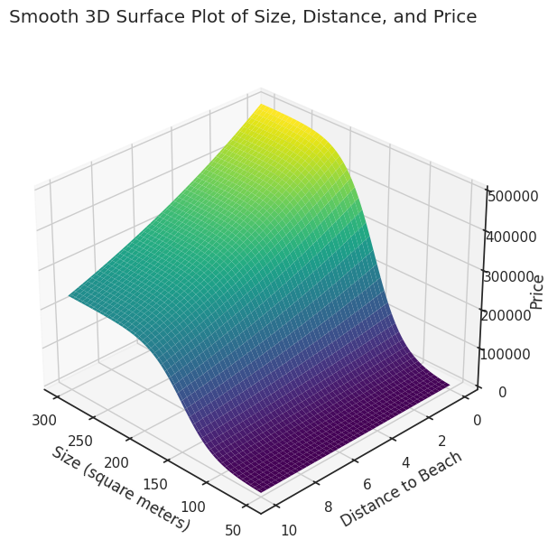
Now consider that you might have 2 houses with the same size and same distance to the beach, yet they sell for different prices. This means the relationship between our variables is not deterministic. For every combination (size, distance, price) we have some probability density of seeing a house with those values in our training data. This is given by the joint probability density function f(X,Y,Z). To visualise this joint density we use a pair plot:
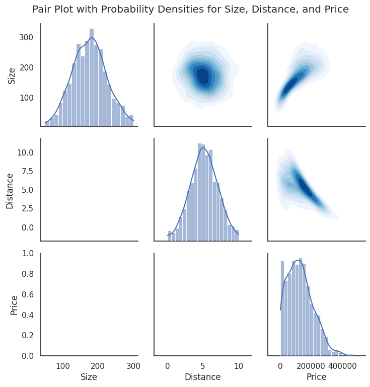
If our only observed variable is size then the relationship to price is not straightforward. For example, suppose we took the average distance to the beach for a house of a certain size. In this case that would be a tricky expected value to calculate. Instead we can use simulations and apply some smoothing to approximate the relationship:
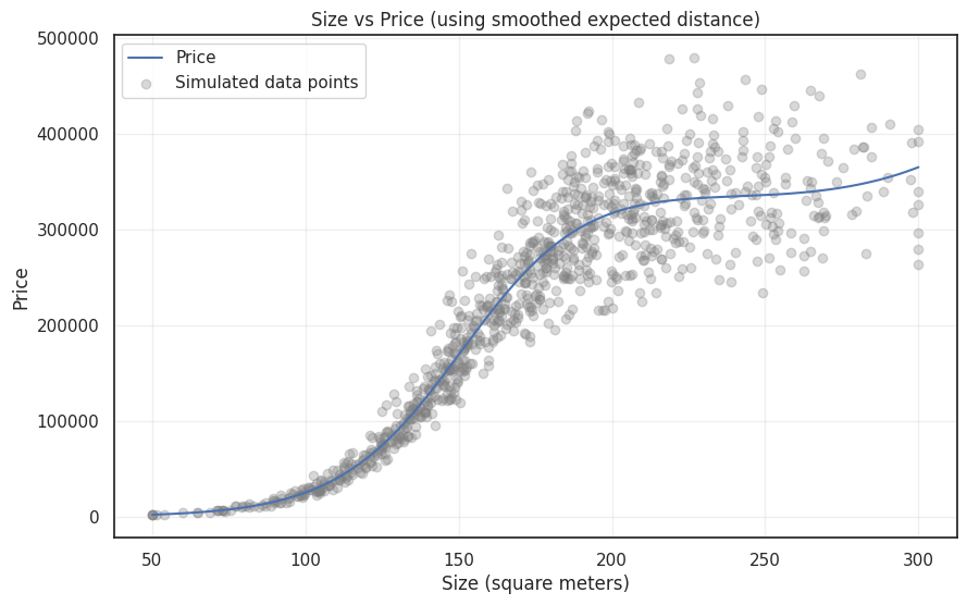
For particularly large houses the effect of distance is compounded. So a large house close to the beach is much more expensive than the same size house further away. Both are expensive but the variance is significantly different at the high-end. This will make it difficult to predict the true shape of the relationship at the tail end.
Additionally, we must consider the endogenous bias in our sample. The probability of being sold (W) is affected by all attributes which we can show in this pair plot:
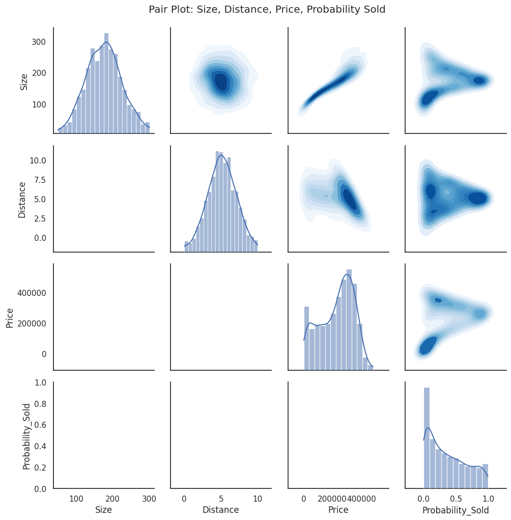
How might we think about this new attribute (W)? Fewer small/large houses are built so fewer are put up for sale. In reality there are many factors that impact whether or not a property is listed for sale including people’s willingness to sell. This endogenous bias affects our probability density function f(X, Z, Y) by making certain combinations less likely without affecting the relationship between variables f*(x,z)=y.
We adjust the pair plot to show the updated relationship between variables given the endogenous bias of seeing a particular house on the market.
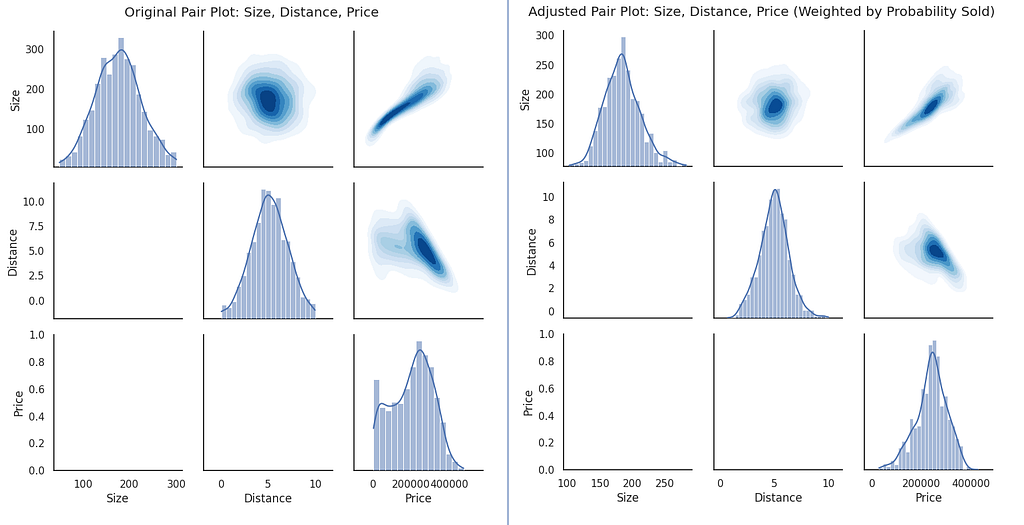
Notice that there is a slight but observable change in the apparent relationship between house size and price.
What does our model capture?
Let’s take another look at the plot which shows the relationship of price and size directly.

When we analyse the bias/variance of a model are we analysing the error against this function? No, we are not. We are building a model of the statistical process which generates our data — a process which includes the endogenous bias. This means the expected error is the expectation over all possible samples from our distribution.
Put another way: the bias-variance trade-off of a regression model concerns the expected error of that model across all possible worlds. Because the expected value is weighed by the probability of seeing particular values it will be affected by endogenous sampling bias.
It feels strange that the probability of a house being sold should influence the calculations we make about the relationship between the size of the house and its sale price. Yet this calculation is at the very heart of the bias-variance trade-off.
Error decomposition of regression
In the German Tank Problem the probability of our sample was conditioned on the value we were trying to predict f(X|N). In regression there’s a joint probability distribution between predictor and target values f(X, Y). This means that the relationship between the variables has some inherent variation which can’t be accounted for. In truth there are probably more latent variables we aren’t considering but that’s a debate for another time. This variability leads to an irreducible error term which is why we describe it as predicting the expected value of y given observations x.
Note that this irreducible error is sometimes called “aleatoric uncertainty”. This is contrasted with “epistemic uncertainty” caused by a lack of knowledge. An under specified model may lead to epistemic uncertainty but even a perfect model has to face aleatoric uncertainty.
This new structure means that the expected MSE is decomposed into bias, variance, and an irreducible error term:
![text{Err} &= mathbb{E}_{x,y}mathbb{E}_{D}left[(y — h(xvert D))² right] \ &= mathbb{E}_{x,y}left[(y — bar{h}(x))² right] + mathbb{E}_{x,y}mathbb{E}_{D}left[(h(xvert D) — bar{h}(x))² right] + epsilon \ &= text{Bias}²(h) + text{Var}(h) + epsilon \ \ & bar{h}(x)=mathbb{E}_{D}[h(xvert D)]](https://cdn-images-1.medium.com/max/772/1*QjhXWQEOZjupQ8xjjIB2Ng.png)
In this decomposition I’m showing again the subscripts for the expectation to clearly show that what each expectation is conditioned on. The new term (h-bar) is the expected value of our model averaged over all possible datasets that could have been used to construct our model. Think of possible worlds in which we collect a training dataset and creating an ensemble model that averages all predictions across all possible worlds.
The expected error of our model needs to be an integral over:
- All possible data sets (D) we could use to train our model (h)
- All possible values of x ∈ X (weighted by their marginal probabilities)
- All possible values of y ∈ Y (similarly weighted)
![text{Err} &= mathbb{E}_{x,y}mathbb{E}_{D}left[(y — h(xvert D))² right] \ &= int_{xin X} int_{yin Y} int_{D} P(x)P(y)P(D)(y-h(xvert D))² dx , dy , dD](https://cdn-images-1.medium.com/max/785/1*7qReKAr2DyrEW0HwMaQ7Uw.png)
Interestingly it’s also the expectation over a fixed size training set — the fact that sample size might be dependent on the variables isn’t captured in this decomposition.
More importantly this integral is completely intractable for our problem. In fact calculating the expected error is generally intractable for non-trivial problems. This is true even knowing the real process used to generate this synthetic data. Instead we’re going to run some simulations using different samples and average out the errors to see how different models perform.
Model complexity
If you know anything about the bias-variance trade-off then you probably know bias comes from “underfitting” and variance comes from “overfitting”. It’s not immediately obvious why a model which overfits should have low bias, or why a model which underfits should have low variance. These terms are typically associated with model complexity, but what exactly does it mean?
Here are 6 possible worlds in which 35 houses were put on sale. In each instance we use polynomial regression to fit terms from [x⁰…x⁵] and we compare the predicted polynomial against the true expected price for that size. Notice how different training samples create wildly different polynomial predictions:
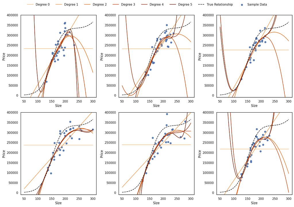
But remember — in terms of the bias-variance trade-off we are not evaluating our model against the true relationship. That true relationship ignores the endogenous sampling bias. Instead we can adjust the “true” relationship based on the effects of W to factor in the probability of being sold. Now we can see predictions that match closer to the adjusted true relationship:
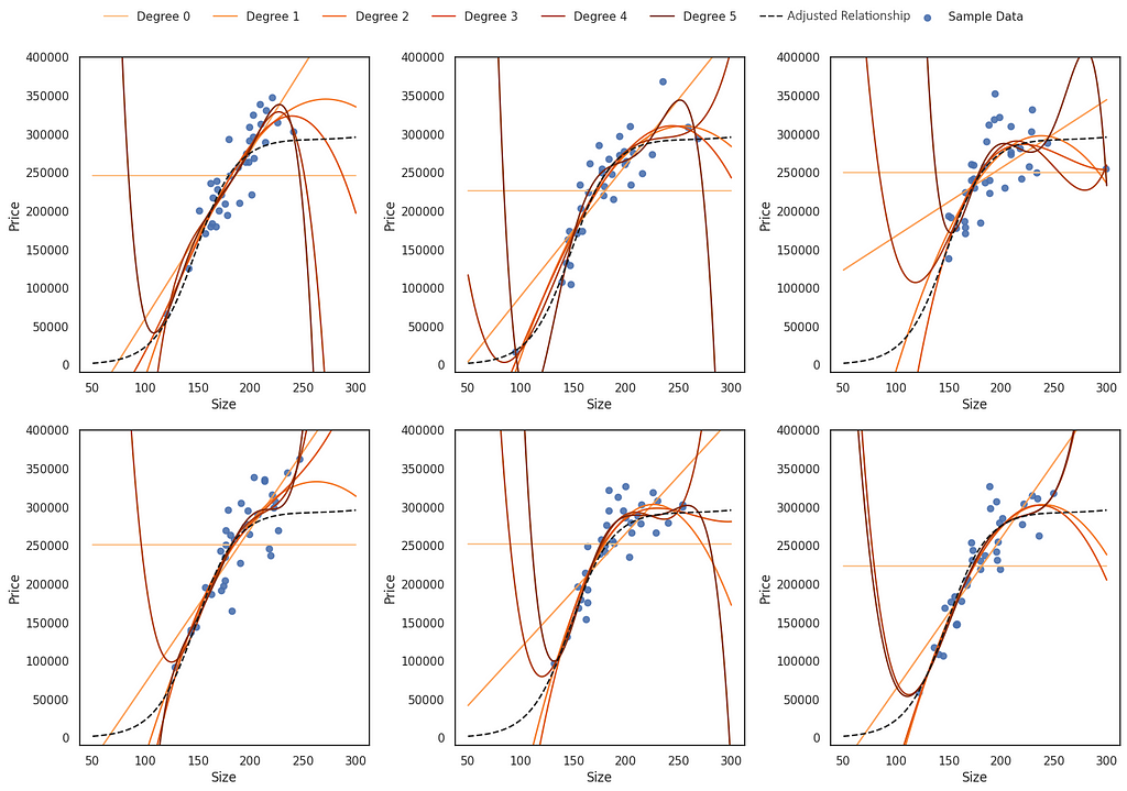
We can find the expected value of predictions by simulating 1,000 possible worlds. This is the expected prediction for each polynomial degree based on the size of the house:
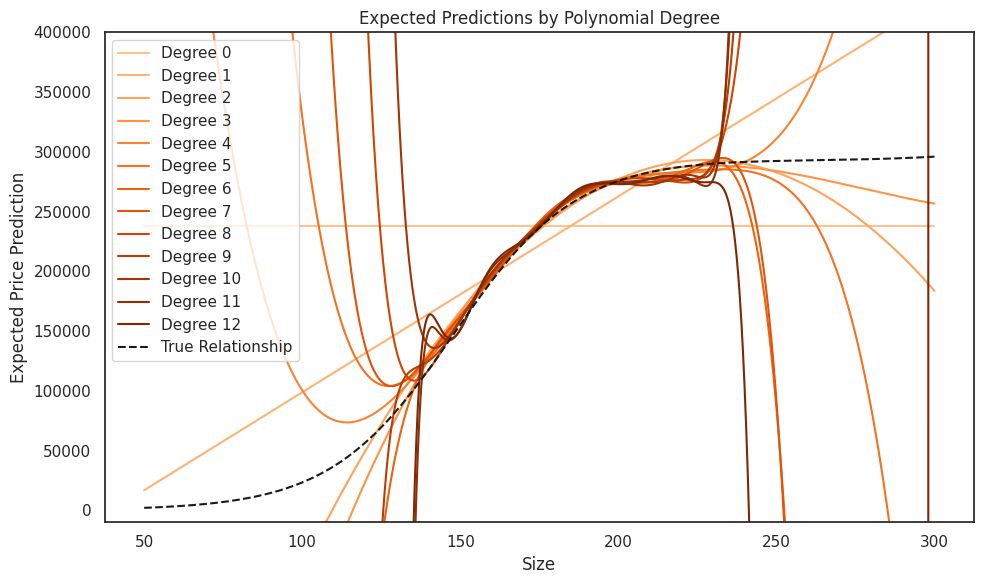
Notice how these models do particularly poorly at the low end. This is entirely due to the endogenous sampling bias because we are unlikely to see many particularly small houses for sale. Also notice that the models tend to do poorly for particularly large houses, which has a combined effect from both the endogenous sampling bias and the latent variable.
Now we take the model function h and include an additional term λ which represents the hyperparameters used for a particular class of models. Rather than polynomial degree we’ll have λ represent the subset for the number of polynomial terms being used. For our simulations we’ll do a brute force check of all combinations up 5 terms with a polynomial degree of 10 and select the ones with the best training error. Ideally this would be done with cross-validation but we’ll skip this as it’s not a useful technique in deep learning. Also note that with 5 terms and 1000 simulations a brute force search is already quite slow.
Next we introduce a function g(λ)=c which represents the “complexity” of the model based on the hyperparameters selected. In this case g is just the identity function and the complexity is entirely concerned with the subset of polynomial terms used.
The expected error of a fixed model architecture with varying complexity is given by:
![text{Err}(lambda) &= mathbb{E}_{x,y}mathbb{E}_p left[ (y — h(x vert D, lambda))² right] \
&= text{Bias}²(h, lambda) + text{Var}(h, lambda) + epsilon \
text{Err}( c) &= mathbb{E}_{x,y}mathbb{E}_p left[ (y — h(x vert D, g^{-1}( c)))² right] \
&= text{Bias}²(h, g^{-1}( c)) + text{Var}(h, g^{-1}( c)) + epsilon](https://cdn-images-1.medium.com/max/618/1*pMEJJ_t3enbQLjDjcAweag.png)
Now instead of calculating the expected prediction by polynomial degree we instead use the subset selection size. Averaged over 1,000 simulations we get the following predictions:
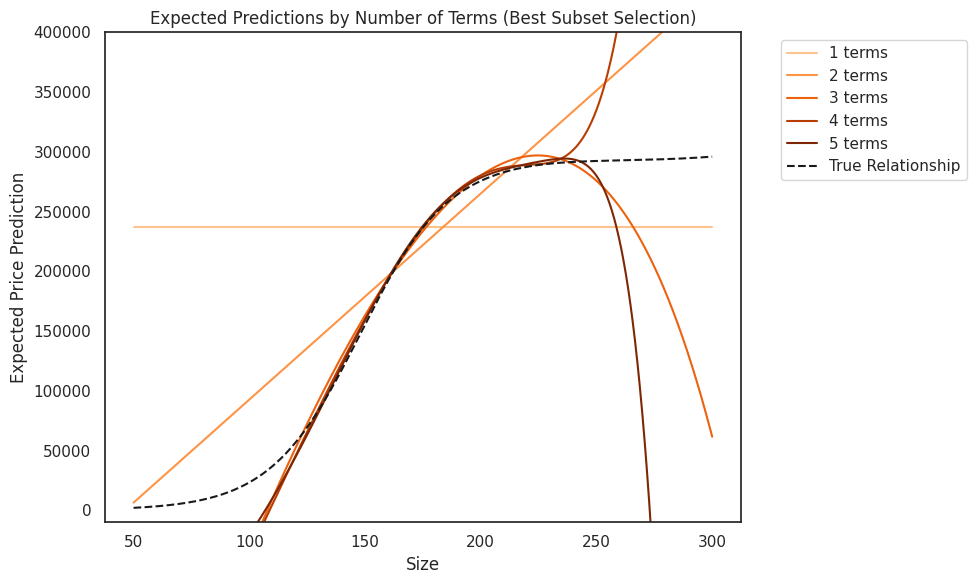
Further, we can plot the total expected error (weighted by probability of seeing a house of that size) and decompose the error into a bias and variance term:
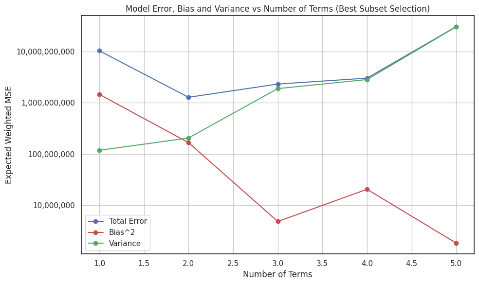
Once again remember that to get the expected error we are averaging over all possible worlds. We can see that:
- Bias² decreases as the model complexity increases.
- Variance increases as the model complexity increases.
- The total error decreases, hits a minimum point, and then rises.
- In this problem the total error also has a strong contribution from the irreducible error.
Using some assumptions we can identify some attributes of the expected error for any model h. The core assumptions are:
- At low complexity the total error is dominated by bias, while at high complexity total error is dominated by variance. With bias ≫ variance at the minimum complexity and variance ≫ bias at high complexity.
- As a function of complexity, bias is monotonically decreasing and variance is monotonically increasing.
- The complexity function g is differentiable.
Based on these assumptions we can expect most models to behave similarly to the plot above. First the total error drops to some optimal point and then it starts to increase as increased complexity leads to more variance. To find the optimal complexity we start by taking the partial derivative of our error decomposition with respect to the complexity:
![&frac{partial}{partial c} left[ text{Bias}²(h, g^{-1}( c )) + text{Var}(h, g^{-1}( c )) + epsilon right] \ & text{let } text{BiasT}=text{Bias}² \ &=frac{partial}{partial c} left[ text{BiasT}(h, g^{-1}( c )) + text{Var}(h, g^{-1}( c )) + epsilon right] \ &=text{BiasT}’(h, g^{-1}( c )) cdot frac{partial}{partial c} g^{-1}( c ) + text{Var}’(h, g^{-1}( c )) cdot frac{partial}{partial c} g^{-1}( c )](https://cdn-images-1.medium.com/max/791/1*176lkQIRgMFkklR6IFNsog.png)
The inflection point happens when the partial derivative is 0.

At the optimal point the derivative of the bias² is the negative of the variance. And without further assumptions that’s actually all we can say about the optimal error. For example, here are random bias and variance functions which happen to meet the assumptions listed. The point at which their derivatives are inverses of each other is the point at which the total error is minimised:
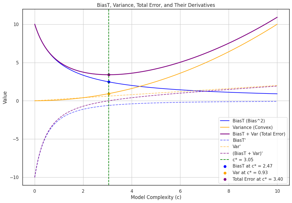
If we add an extra assumption that bias and variance are symmetric around the optimal point then we can narrow down the lowest error to be at Bias²(c*)=Var(c*). If you play around with a few options you will notice that the optimal point tends to be near the point at which bias² and variance terms are equal. But without the added assumption that’s not guaranteed.
Implications
We know that calculating the optimal point is intractable. But it’s generally understood that low bias inherently leads to exploding variance due to the impacts of model complexity. Think about that for a moment: the implication is that you can’t have a model that both performs well and is unbiased.
Generalisation error
Because we can’t literally average over all possible worlds we need some other way of calculating the the total expected error of our model. The Generalisation error captures the performance of a model on unseen data. It’s the gap between how well a model fits its training data and how well it performs on the underlying data distribution. For an arbitrary loss function ℓ we can state the generalisation error as:
![text{Err}_text{gen} &= mathbb{E}_{x,y} left[ ell left( h(x vert D, lambda), y right) right]](https://cdn-images-1.medium.com/max/396/1*YTrKV0DteBYDl2_EaXTOnQ.png)
Note that even here we can’t possibly calculate the expected performance of our model across all possible combinations of (x,y). We approximate the generalisation error by collecting a new independent dataset to evaluate on. There are different ways we could evaluate performance:
- In-sample error: Training error computed on the data used to fit the model. This is often misleadingly low for overfit models and will not capture generalisation capability.
- Out-of-sample error (OOS): Performance on a held-out sample from the same distribution as our training set. This is the gold standard for assessing generalisation.
- Out-of-distribution error (OOD): The performance on data that does not belong to the training distribution. Think of a house pricing model trained on urban areas tested on rural houses — it’s likely to fail.
These concepts tie into what we’ve already explored in the bias-variance trade-off. Biased models will fail to capture the relationships between the variables and so the relationships they do describe won’t fit on to OOS examples. But high variance models can produce wildly different predictions depending on the sample that they saw. Even though they may have low bias (in expectation) that’s only because the magnitudes of their errors cancel out.
Let’s now consider two concepts closely related to bias and variance:
- Overfitting is best thought of as a consequence of model capacity and training data availability. When a model has too many parameters relative to the size or diversity of the training data, it fits not just the underlying signal but also the noise in the data.
- Underfitting on the other hand is a consequences of underspecification. The model is not sufficiently complex to capture the details of the underlying distribution. This is usually due to too few parameters relative to the complexity of the best fit curve.
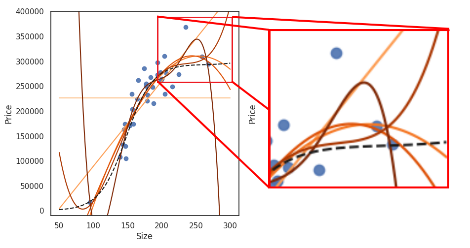
Let’s take a look at one of the possible worlds from our simulation. Here we zoom in on the large-size high-price portion of our sample. Notice how more complex models attempt to draw a curve that essentially connects all of the observed points. If the sample were slightly different the shape of these curves could be wildly different. On the other hand the low complexity models (e.g. the y=mx+b or y=b lines) aren’t able to capture the curvature at the tails of the dataset.
A quick note on regularisation
L1 and L2 regularisation used in Lasso and Ridge regression are techniques that limit the complexity in an interesting way. Instead of reducing the number of parameters they encourage smaller coefficients which in turn produces smoother plots that are less likely to oscillate between points in the training data. This has the effect of reducing model complexity and hence increasing bias. The general idea is that the increase in bias is more than made up for by the reduced variance. Entire textbooks have been written on this topic so I won’t cover regularisation in this article.
Validation and test sets
If there’s one lesson we can take from our exploration of bias, variance, and generalisation error it’s this: models must be evaluated on data they have never seen before. The concept is straightforward, but its application is often misunderstood.
Validation and test sets help mitigate the risk of overfitting by acting as a proxy for real-world performance. Let’s start with a clear distinction:
- Validation set: Used during model development to tune hyperparameters and select the best-performing model variant.
- Test set: A completely held-out dataset used to evaluate the final model after all training and tuning are complete.
The goal of using these sets is to approximate the expected out-of-sample performance. But there’s a catch. If you use the validation set too often, it becomes part of the training process, introducing an unseen data leakage problem. You may “overfit” the hyperparameters to the validation set and so fail to capture the real nature of the relationship. That is why it’s useful to have a separate test set for evaluating the performance of your final model. The performance on the test set acts as a proxy for our total error calculation. The chief problem is: how should we structure our test set?
Tail risks and stratification
Remember that estimation requires knowledge of the distribution’s shape while prediction focuses only on maximizing empirical accuracy. For empirical accuracy we need to think about risk mitigation. An automated algorithm for setting prices may do well in expectation yet pose significant tail risks.
Significantly under-pricing high-end homes would result in opportunistic buyers taking advantage of undervalued assets. Significantly over-pricing high-end homes would result in no one buying. The asymmetry of the real world doesn’t match the symmetry of expected values.
Even though the model performs well in expectation it fails spectacularly when deployed in the real world.
This is why stratification can be a vital component of setting up a test set. This might involve dropping examples from overly dense regions of the sampling space until there’s a uniform distribution across the entire domain. This test set would not be iid to our training data and so it does not measure the generalisation error as described in the equation we saw earlier.
Another option would need to use a different loss function ℓ (i.e. not MSE but one that factors in our risk requirements). This loss function may change the dynamics of the error decomposition and may favour a significantly underfit model.
What does our model say about the real world?
Finally consider what we are trying to achieve. In deep learning we may have the goal of training general purpose agents. What does the bias-variance trade-off tell us about whether or not Large Language Models understand the text they are reading? Nothing. If we want to assess whether or not our training process creates an accurate model of the world we need to consider the out of distribution (OOD) error. For models that have any hope of being general they must work OOD. For that we’ll need to leave the realm of statistics and finally make our way into the territory of machine learning.
Reflection
In the previous section we learned about the core concepts of bias and variance. In this section we had a more complex problem that articulated how bias and variance relate to the expected performance of our model given different training data.
We added some complexity with latent variables affecting our models performance at the tails — leading to potential tail risks. We also had an endogenous sampling bias which meant that an assessment of expected error may not describe the true underlying relationship.
We introduced the idea of validation and test sets as methods for helping determine OOS performance to test our models generalisation error. We also talked about alternative test set constructions that throw away iid assumptions but may result in models with lower tail risks.
We also introduced some key assumptions that aren’t going to apply once we enter the realm of deep learning. Before we get there we’re going to apply all these lessons to design robust machine learning algorithms.
Robust Machine Learning
In deep learning we often deal with large datasets and complicated models. This combination can lead to model training times of many hours (and sometimes even weeks or months). When faced with the reality of hours spent training a single model the prospect of using techniques like cross-validation is daunting. And yet, at the end of the training process we often have strong demands for performance given such a large investment in time and compute.
Two views of robustness
Parts of this section focus on ideas from the paper Machine Learning Robustness: A Primer. Robust models are described as ones which continue to perform well when deployed despite encountering inputs which may be different to their training observations. They provide the following useful examples of how inputs can change in production:
Examples of variations and changes in the input data:
— Variations in input features or object recognition patterns that challenge the inductive bias learned by the model from the training data.
— Production data distribution shifts due to naturally occurring distortions, such as lighting conditions or other environmental factors.
— Malicious input alterations that are deliberately introduced by an attacker to fool the model or even steer its prediction in a desired direction.
— Gradual data drift resulting from external factors, such as evolution in social behavior and economic conditions.
Examples of model flaws and threats to stable predictive performance:
— Exploitation of irrelevant patterns and spurious correlations that will not hold up in production settings.
— Difficulty in adapting to edge-case scenarios that are often underrepresented by training samples.
— Susceptibility to adversarial attacks and data poisonings that target the vulnerabilities of overparametrized modern ML models.
— Inability of the model to generalize well to gradually-drifted data, leading to concept drift as its learned concepts become obsolete or less representative of the current data distribution.
We’re going to contrast that with the paper A Mathematical Foundation for Robust Machine Learning based on Bias-Variance Trade-off. Note that this paper was withdrawn because “several theorem and propositions that are highly-related were not mentioned”. However, it still provides an effective overview of robustness from the perspective of the bias-variance trade-off. We’ll look at this paper first and consider how the shape of the decision boundary of a model is affected by complexity and training data.
Error decomposition for classification
In binary classification we train a model to predict a probability for class 1 (vs class 0). This represents the expected value for the target variable (y∈{0,1}) given observation x. The total error is the difference between the predicted probability and the expected error. The loss for a single item is most simply measured as:

This effectively measures the distance of the predicted probability from the true class and dynamically adjusts based on whether the true class is equal to 0 or 1.
We note that the bias-variance decomposition for classification is more complicated. In the section on the German Tank Problem I pointed out that a biased model may still be correct because the variance could (by chance) push the prediction closer to the truth. When using the squared loss this is completely cancelled out by the fact that the expected loss increases much more for highly incorrect estimates. So any potential benefit from high variance is overshadowed by estimates which are significantly off target.
In the binary classification case this is not necessarily true. Bias, variance, and total error must be in the range (0,1). If the model is completely biased (bias=1) then the model always predicts the wrong class in expectation. Any variance actually makes the correct prediction more likely! Hence, in this particular scenario Err=Bias-Var.
If we add a reasonable assumption that the sum of the bias and variance must be less than or equal to 1 we get the standard decomposition except that the total error is simply Err=Bias+Var rather than Bias².
Model complexity is complicated
In deep learning you might think that model complexity is entirely concerned with the number of parameters in the network. But consider that neural networks are trained with stochastic gradient descent and take time to converge on a solution. In order for the model to overfit it needs time to learn a transformation connecting all of the training data points. So model complexity is not just a function of number of parameters but also of the number of epochs training on the same set of data.
This means our function g(λ)=c is not straightforward as with the case of polynomial regression. Additionally techniques like early stopping explicitly address the variance of our model by stopping training once error rates start to increase on a validation set.
According to the paper are 3 main types of hyperparameters that affect bias and variance:
- Type I: A hyperparameter is used to balance bias and variance directly (e.g. as the weight applied to a regularisation term like weight decay).
- Type II: Indirectly affecting bias and variance by adjusting the loss signal from individual training examples (e.g. reducing or increasing the penalty for large prediction errors).
- Type III: Control parts of the training procedure which affect model complexity (e.g. number of epochs training a neural network, early stopping, or the depth of a decision tree).
Easy vs hard examples
A dataset is considered “harder” to learn from if a model has a larger expected generalisation error when trained on that dataset. Formally:

Note: “for all λ” is a strong condition that may not always hold. A dataset may be harder to learn from under some hyperparameters but not others.
We make an assumption that the optimal complexity (c*) for the harder dataset is greater than the optimal complexity of an easier dataset. We can plot the expected error of models trained on the two dataset like this:
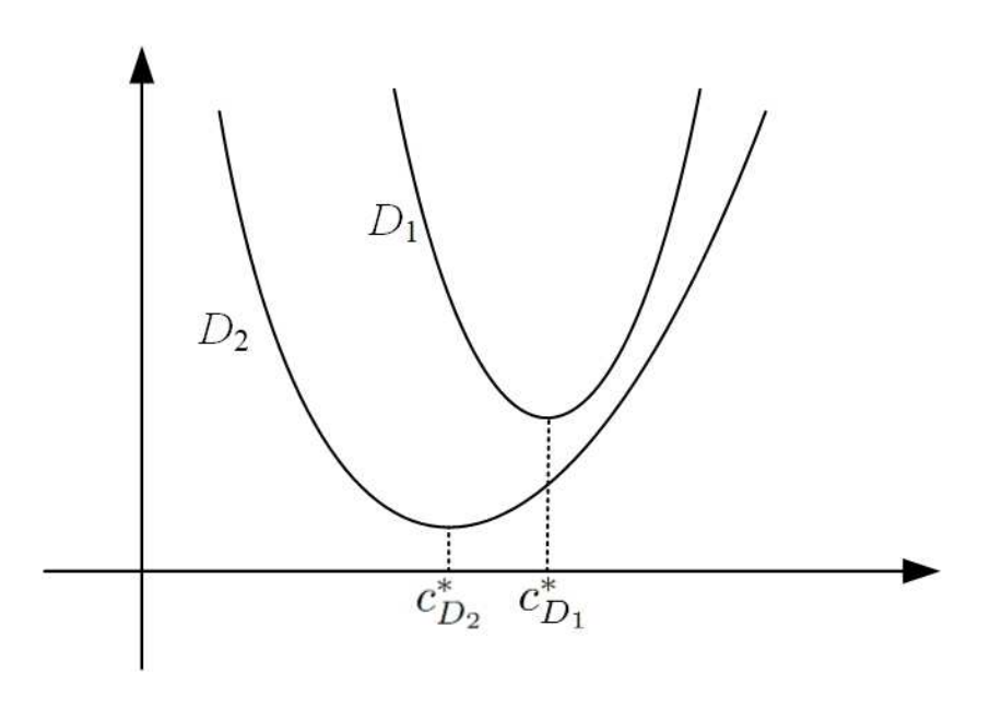
If we partition the training data into “easy” and “hard” subsets we can use similar logic to conclude that a subset of the data is harder to learn from. This can be extended to classify an individual example (x,y) as easy or hard. Consider the reasons that an example might be hard to learn from:
- Noisy labels (i.e. badly annotated data)
- Sparse region of the feature space
- A necessarily complex classification boundary
Now consider the focal loss which is expressed as:

This is similar to using a loss weighting on specific examples to give the model a stronger learning signal in trickier parts of the feature space. One common weighting method is to weight by inverse frequency which gives a higher loss to examples of the sparser class. The focal loss has the effect of automatically determining what makes an example hard based on the current state of the model. The model’s current confidence is used to dynamically adjust the loss in difficult regions of the feature space. So if the model is overly confident and incorrect, that sends a stronger signal than if the model is confident but correct.
The weighting parameter γ is an example of a Type II hyperparameter which adjusts the loss signal from training examples. If an example is hard to learn from then focal loss would ideally encourage the model to become more complex in that part of the feature space. Yet there are many reasons an example may be hard to learn from so this is not always desirable.
Shape of the decision boundary
Here I’ve created a 2D dataset with simple shapes in repeated patterns acting as a decision boundary. I’ve also added a few “dead zones” where data is much harder to sample. With ~100,000 data points a human can look at the plot and quickly see what the boundaries should be.
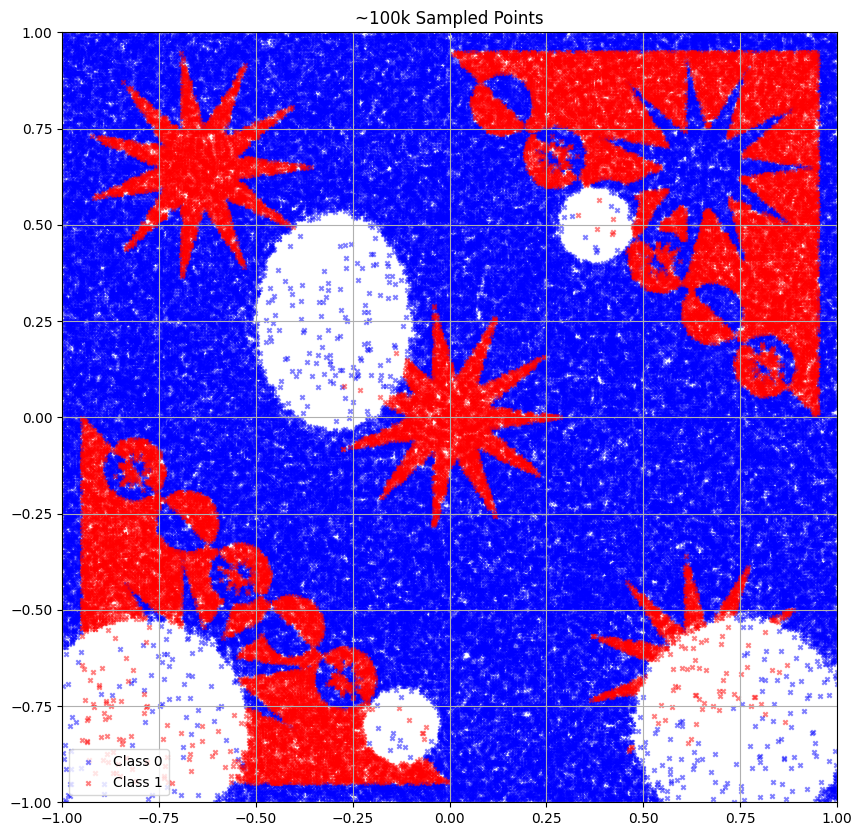
Despite the dead zones you can easily see the boundary because billions of years of natural selection have equipped you with general pattern recognition capabilities. It will not be so easy for a neural network trained from scratch. For this exercise we won’t apply explicit regularisation (weight decay, dropout) which would discourage it from overfitting the training data. Yet it’s worth noting that layer norm, skip connections, and even stochastic gradient descent can act as implicit regularisers.
Here the number of parameters (p) is roughly equal to the number of examples (N). We’ll focus only on the training loss to observe how the model overfits. The following 2 models are trained with fairly large batch sizes for 3000 epochs. The predicted boundary from the model on the left uses a standard binary cross entropy loss while the one on the right uses the focal loss:

The first thing to notice is that even though there’s no explicit regularisation there are relatively smooth boundaries. For example, in the top left there happened to be a bit of sparse sampling (by chance) yet both models prefer to cut off one tip of the star rather than predicting a more complex shape around the individual points. This is an important reminder that many architectural decisions act as implicit regularisers.
From our analysis we would expect focal loss to predict complicated boundaries in areas of natural complexity. Ideally, this would be an advantage of using the focal loss. But if we inspect one of the areas of natural complexity we see that both models fail to identify that there is an additional shape inside the circles.
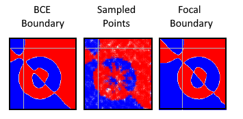
In regions of sparse data (dead zones) we would expect focal loss to create more complex boundaries. This isn’t necessarily desirable. If the model hasn’t learned any of the underlying patterns of the data then there are infinitely many ways to draw a boundary around sparse points. Here we can contrast two sparse areas and notice that focal loss has predicted a more complex boundary than the cross entropy:
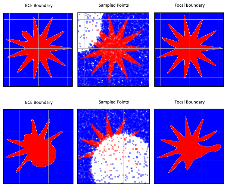
The top row is from the central star and we can see that the focal loss has learned more about the pattern. The predicted boundary in the sparse region is more complex but also more correct. The bottom row is from the lower right corner and we can see that the predicted boundary is more complicated but it hasn’t learned a pattern about the shape. The smooth boundary predicted by BCE might be more desirable than the strange shape predicted by focal loss.
This qualitative analysis doesn’t help in determining which one is better. How can we quantify it? The two loss functions produce different values that can’t be compared directly. Instead we’re going to compare the accuracy of predictions. We’ll use a standard F1 score but note that different risk profiles might prefer extra weight on recall or precision.
To assess generalisation capability we use a validation set that’s iid with our training sample. We can also use early stopping to prevent both approaches from overfitting. If we compare the validation losses of the two models we see a slight boost in F1 scores using focal loss vs binary cross entropy.
- BCE Loss: 0.936 (Validation F1)
- Focal Loss: 0.954 (Validation F1)
So it seems that the model trained with focal loss performs slightly better when applied on unseen data. So far, so good, right?
The trouble with iid generalisation
In the standard definition of generalisation, future observations are assumed to be iid with our training distribution. But this won’t help if we want our model to learn an effective representation of the underlying process that generated the data. In this example that process involves the shapes and the symmetries that determine the decision boundary. If our model has an internal representation of those shapes and symmetries then it should perform equally well in those sparsely sampled “dead zones”.
Neither model will ever work OOD because they’ve only seen data from one distribution and cannot generalise. And it would be unfair to expect otherwise. However, we can focus on robustness in the sparse sampling regions. In the paper Machine Learning Robustness: A Primer, they mostly talk about samples from the tail of the distribution which is something we saw in our house prices models. But here we have a situation where sampling is sparse but it has nothing to do with an explicit “tail”. I will continue to refer to this as an “endogenous sampling bias” to highlight that tails are not explicitly required for sparsity.
In this view of robustness the endogenous sampling bias is one possibility where models may not generalise. For more powerful models we can also explore OOD and adversarial data. Consider an image model which is trained to recognise objects in urban areas but fails to work in a jungle. That would be a situation where we would expect a powerful enough model to work OOD. Adversarial examples on the other hand would involve adding noise to an image to change the statistical distribution of colours in a way that’s imperceptible to humans but causes miss-classification from a non-robust model. But building models that resist adversarial and OOD perturbations is out of scope for this already long article.
Robustness to perturbation
So how do we quantify this robustness? We’ll start with an accuracy function A (we previously used the F1 score). Then we consider a perturbation function φ which we can apply on both individual points or on an entire dataset. Note that this perturbation function should preserve the relationship between predictor x and target y. (i.e. we are not purposely mislabelling examples).
Consider a model designed to predict house prices in any city, an OOD perturbation may involve finding samples from cities not in the training data. In our example we’ll focus on a modified version of the dataset which samples exclusively from the sparse regions.
The robustness score (R) of a model (h) is a measure of how well the model performs under a perturbed dataset compared to a clean dataset:

Consider the two models trained to predict a decision boundary: one trained with focal loss and one with binary cross entropy. Focal loss performed slightly better on the validation set which was iid with the training data. Yet we used that dataset for early stopping so there is some subtle information leakage. Let’s compare results on:
- A validation set iid to our training set and used for early stopping.
- A test set iid to our training set.
- A perturbed (φ) test set where we only sample from the sparse regions I’ve called “dead zones”.
| Loss Type  | Val (iid) F1  | Test (iid) F1   | Test (φ) F1 |   R(φ)  |
|------------|---------------|-----------------|-------------|---------|
| BCE Loss   |    0.936      |    0.959        |   0.834     | 0.869   |
| Focal Loss |    0.954      |    0.941        |   0.822     | 0.874   |
The standard bias-variance decomposition suggested that we might get more robust results with focal loss by allowing increased complexity on hard examples. We knew that this might not be ideal in all circumstances so we evaluated on a validation set to confirm. So far so good. But now that we look at the performance on a perturbed test set we can see that focal loss performed slightly worse! Yet we also see that focal loss has a slightly higher robustness score. So what is going on here?
I ran this experiment several times, each time yielding slightly different results. This was one surprising instance I wanted to highlight. The bias-variance decomposition is about how our model will perform in expectation (across different possible worlds). By contrast this robustness approach tells us how these specific models perform under perturbation. But we made need more considerations for model selection.
There are a lot of subtle lessons in these results:
- If we make significant decisions on our validation set (e.g. early stopping) then it becomes vital to have a separate test set.
- Even training on the same dataset we can get varied results. When training neural networks there are multiple sources of randomness to consider which will become important in the last part of this article.
- A weaker model may be more robust to perturbations. So model selection needs to consider more than just the robustness score.
- We may need to evaluate models on multiple perturbations to make informed decisions.
Comparing approaches to robustness
In one approach to robustness we consider the impact of hyperparameters on model performance through the lens of the bias-variance trade-off. We can use this knowledge to understand how different kinds of training examples affect our training process. For example, we know that miss-labelled data is particularly bad to use with focal loss. We can consider whether particularly hard examples could be excluded from our training data to produce more robust models. And we can better understand the role of regularisation by consider the types of hyperparameters and how they impact bias and variance.
The other perspective largely disregards the bias variance trade-off and focuses on how our model performs on perturbed inputs. For us this meant focusing on sparsely sampled regions but may also include out of distribution (OOD) and adversarial data. One drawback to this approach is that it is evaluative and doesn’t necessarily tell us how to construct better models short of training on more (and more varied) data. A more significant drawback is that weaker models may exhibit more robustness and so we can’t exclusively use robustness score for model selection.
Regularisation and robustness
If we take the standard model trained with cross entropy loss we can plot the performance on different metrics over time: training loss, validation loss, validation_φ loss, validation accuracy, and validation_φ accuracy. We can compare the training process under the presence of different kinds of regularisation to see how it affects generalisation capability.
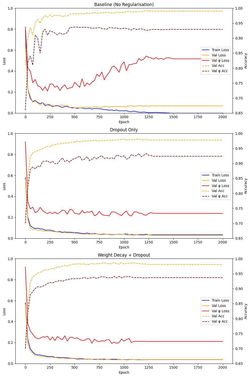
In this particular problem we can make some unusual observations
- As we would expect without regularisation, as the training loss tends towards 0 the validation loss starts to increase.
- The validation_φ loss increases much more significantly because it only contains examples from the sparse “dead zones”.
- But the validation accuracy doesn’t actually get worse as the validation loss increases. What is going on here? This is something I’ve actually seen in real datasets. The model’s accuracy improves but it also becomes increasingly confident in its outputs, so when it is wrong the loss is quite high. Using the model’s probabilities becomes useless as they all tend to 99.99% regardless of how well the model does.
- Adding regularisation prevents the validation losses from blowing up as the training loss cannot go to 0. However, it can also negatively impact the validation accuracy.
- Adding dropout and weight decay is better than just dropout, but both are worse than using no regularisation in terms of accuracy.
Reflection
If you’ve stuck with me this far into the article I hope you’ve developed an appreciation for the limitations of the bias-variance trade-off. It will always be useful to have an understanding of the typical relationship between model complexity and expected performance. But we’ve seen some interesting observations that challenge the default assumptions:
- Model complexity can change in different parts of the feature space. Hence, a single measure of complexity vs bias/variance doesn’t always capture the whole story.
- The standard measures of generalisation error don’t capture all types of generalisation, particularly lacking in robustness under perturbation.
- Parts of our training sample can be harder to learn from than others and there are multiple ways in which a training example can be considered “hard”. Complexity might be necessary in naturally complex regions of the feature space but problematic in sparse areas. This sparsity can be driven by endogenous sampling bias and so comparing performance to an iid test set can give false impressions.
- As always we need to factor in risk and risk minimisation. If you expect all future inputs to be iid with the training data it would be detrimental to focus on sparse regions or OOD data. Especially if tail risks don’t carry major consequences. On the other hand we’ve seen that tail risks can have unique consequences so it’s important to construct an appropriate test set for your particular problem.
- Simply testing a model’s robustness to perturbations isn’t sufficient for model selection. A decision about the generalisation capability of a model can only be done under a proper risk assessment.
- The bias-variance trade-off only concerns the expected loss for models averaged over possible worlds. It doesn’t necessarily tell us how accurate our model will be using hard classification boundaries. This can lead to counter-intuitive results.
Deep Learning and Over-parametrisation
Let’s review some of the assumptions that were key to our bias-variance decomposition:
- At low complexity, the total error is dominated by bias, while at high complexity total error is dominated by variance. With bias ≫ variance at the minimum complexity.
- As a function of complexity bias is monotonically decreasing and variance is monotonically increasing.
- The complexity function g is differentiable.
It turns out that with sufficiently deep neural networks those first two assumptions are incorrect. And that last assumption may just be a convenient fiction to simplify some calculations. We won’t question that one but we’ll be taking a look at the first two.
Let’s briefly review what it means to overfit:
- A model overfits when it fails to distinguish noise (aleatoric uncertainty) from intrinsic variation. This means that a trained model may behave wildly differently given different training data with different noise (i.e. variance).
- We notice a model has overfit when it fails to generalise to an unseen test set. This typically means performance on test data that’s iid with the training data. We may focus on different measures of robustness and so craft a test set which is OOS, stratified, OOD, or adversarial.
We’ve so far assumed that the only way to get truly low bias is if a model is overly complex. And we’ve assumed that this complexity leads to high variance between models trained on different data. We’ve also established that many hyperparameters contribute to complexity including the number of epochs of stochastic gradient descent.
Overparameterisation and memorisation
You may have heard that a large neural network can simply memorise the training data. But what does that mean? Given sufficient parameters the model doesn’t need to learn the relationships between features and outputs. Instead it can store a function which responds perfectly to the features of every training example completely independently. It would be like writing an explicit if statement for every combination of features and simply producing the average output for that feature. Consider our decision boundary dataset where every example is completely separable. That would mean 100% accuracy for everything in the training set.
If a model has sufficient parameters then the gradient descent algorithm will naturally use all of that space to do such memorisation. In general it’s believed that this is much simpler than finding the underlying relationship between the features and the target values. This is considered the case when p ≫ N (the number of trainable parameters is significantly larger than the number of examples).
But there are 2 situations where a model can learn to generalise despite having memorised training data:
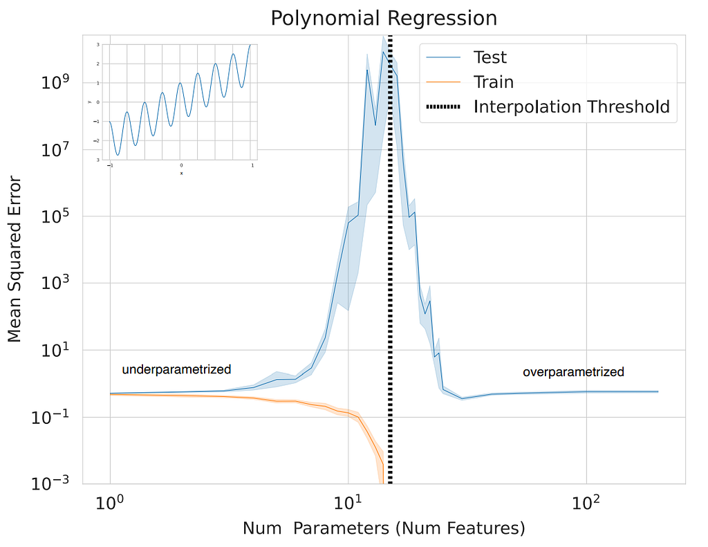
- Having too few parameters leads to weak models. Adding more parameters leads to a seemingly optimal level of complexity. Continuing to add parameters makes the model perform worse as it starts to fit to noise in the training data. Once the number of parameters exceeds the number of training examples the model may start to perform better. Once p ≫ N the model reaches another optimal point.
- Train a model until the training and validation losses begin to diverge. The training loss tends towards 0 as the model memorises the training data but the validation loss blows up and reaches a peak. After some (extended) training time the validation loss starts to decrease.
This is known as the “double descent” phenomena where additional complexity actually leads to better generalisation.
Does double descent require mislabelling?
One general consensus is that label noise is sufficient but not necessary for double descent to occur. For example, the paper Unravelling The Enigma of Double Descent found that overparameterised networks will learn to assign the mislabelled class to points in the training data instead of learning to ignore the noise. However, a model may “isolate” these points and learn general features around them. It mainly focuses on the learned features within the hidden states of neural networks and shows that separability of those learned features can make labels noisy even without mislabelling.
The paper Double Descent Demystified describes several necessary conditions for double descent to occur in generalised linear models. These criteria largely focus on variance within the data (as opposed to model variance) which make it difficult for a model to correctly learn the relationships between predictor and target variables. Any of these conditions can contribute to double descent:
- The presence of singular values.
- That the test set distribution is not effectively captured by features which account for the most variance in the training data.
- A lack of variance for a perfectly fit model (i.e. a perfectly fit model seems to have no aleatoric uncertainty).
This paper also captures the double descent phenomena for a toy problem with this visualisation:
By contrast the paper Understanding Double Descent Requires a Fine-Grained Bias-Variance Decomposition gives a detailed mathematical breakdown of different sources of noise and their impact on variance:
- Sampling — the general idea that fitting a model to different datasets leads to models with different predictions (V_D)
- Optimisation — the effects of parameters initialisation but potentially also the nature of stochastic gradient descent (V_P).
- Label noise — generally mislabelled examples (V_ϵ).
- The potential interactions between the 3 sources of variance.
The paper goes on to show that some of these variance terms actually contribute to the total error as part of a model’s bias. Additionally, you can condition the expectation calculation first on V_D or V_P and it means you reach different conclusions depending on how you do the calculation. A proper decomposition involves understanding how the total variance comes together from interactions between the 3 sources of variance. The conclusion is that while label noise exacerbates double descent it is not necessary.
Regularisation and double descent
Another consensus from these papers is that regularisation may prevent double descent. But as we saw in the previous section that does not necessarily mean that the regularised model will generalise better to unseen data. It more seems to be the case that regularisation acts as a floor for the training loss, preventing the model from taking the training loss arbitrarily low. But as we know from the bias-variance trade-off, that could limit complexity and introduce bias to our models.
Reflection
Double descent is an interesting phenomenon that challenges many of the assumptions used throughout this article. We can see that under the right circumstances increasing complexity doesn’t necessarily degrade a model’s ability to generalise.
Should we think of highly complex models as special cases or do they call into question the entire bias-variance trade-off. Personally, I think that the core assumptions hold true in most cases and that highly complex models are just a special case. I think the bias-variance trade-off has other weaknesses but the core assumptions tend to be valid.
Conclusion
The bias-variance trade-off is relatively straightforward when it comes to statistical inference and more typical statistical models. I didn’t go into other machine learning methods like decisions trees or support vector machines, but much of what we’ve discussed continues to apply there. But even in these settings we need to consider more factors than how well our model may perform if averaged over all possible worlds. Mainly because we’re comparing the performance against future data assumed to be iid with our training set.
Even if our model will only ever see data that looks like our training distribution we can still face large consequences with tail risks. Most machine learning projects need a proper risk assessment to understand the consequences of mistakes. Instead of evaluating models under iid assumptions we should be constructing validation and test sets which fit into an appropriate risk framework.
Additionally, models which are supposed to have general capabilities need to be evaluated on OOD data. Models which perform critical functions need to be evaluated adversarially. It’s also worth pointing out that the bias-variance trade-off isn’t necessarily valid in the setting of reinforcement learning. Consider the alignment problem in AI safety which considers model performance beyond explicitly stated objectives.
We’ve also seen that in the case of large overparameterised models the standard assumptions about over- and underfitting simply don’t hold. The double descent phenomena is complex and still poorly understood. Yet it holds an important lesson about trusting the validity of strongly held assumptions.
For those who’ve continued this far I want to make one last connection between the different sections of this article. In the section in inferential statistics I explained that Fisher information describes the amount of information a sample can contain about the distribution the sample was drawn from. In various parts of this article I’ve also mentioned that there are infinitely many ways to draw a decision boundary around sparsely sampled points. There’s an interesting question about whether there’s enough information in a sample to draw conclusions about sparse regions.
In my article on why scaling works I talk about the concept of an inductive prior. This is something introduced by the training process or model architecture we’ve chosen. These inductive priors bias the model into making certain kinds of inferences. For example, regularisation might encourage the model to make smooth rather than jagged boundaries. With a different kind of inductive prior it’s possible for a model to glean more information from a sample than would be possible with weaker priors. For example, there are ways to encourage symmetry, translation invariance, and even detecting repeated patterns. These are normally applied through feature engineering or through architecture decisions like convolutions or the attention mechanism.
Afterword
I first started putting together the notes for this article over a year ago. I had one experiment where focal loss was vital for getting decent performance from my model. Then I had several experiments in a row where focal loss performed terribly for no apparent reason. I started digging into the bias-variance trade-off which led me down a rabbit hole. Eventually I learned more about double descent and realised that the bias-variance trade-off had a lot more nuance than I’d previously believed. In that time I read and annotated several papers on the topic and all my notes were just collecting digital dust.
Recently I realised that over the years I’ve read a lot of terrible articles on the bias-variance trade-off. The idea I felt was missing is that we are calculating an expectation over “possible worlds”. That insight might not resonate with everyone but it seems vital to me.
I also want to comment on a popular visualisation about bias vs variance which uses archery shots spread around a target. I feel that this visual is misleading because it makes it seem that bias and variance are about individual predictions of a single model. Yet the math behind the bias-variance error decomposition is clearly about performance averaged across possible worlds. I’ve purposely avoided that visualisation for that reason.
I’m not sure how many people will make it all the way through to the end. I put these notes together long before I started writing about AI and felt that I should put them to good use. I also just needed to get the ideas out of my head and written down. So if you’ve reached the end I hope you’ve found my observations insightful.
References
[1] “German tank problem,” Wikipedia, Nov. 26, 2021. https://en.wikipedia.org/wiki/German_tank_problem
[2] Wikipedia Contributors, “Minimum-variance unbiased estimator,” Wikipedia, Nov. 09, 2019. https://en.wikipedia.org/wiki/Minimum-variance_unbiased_estimator
[3] “Likelihood function,” Wikipedia, Nov. 26, 2020. https://en.wikipedia.org/wiki/Likelihood_function
[4] “Fisher information,” Wikipedia, Nov. 23, 2023. https://en.wikipedia.org/wiki/Fisher_information
[5] Why, “Why is using squared error the standard when absolute error is more relevant to most problems?,” Cross Validated, Jun. 05, 2020. https://stats.stackexchange.com/questions/470626/w (accessed Nov. 26, 2024).
[6] Wikipedia Contributors, “Bias–variance tradeoff,” Wikipedia, Feb. 04, 2020. https://en.wikipedia.org/wiki/Bias%E2%80%93variance_tradeoff
[7] B. Efron, “Prediction, Estimation, and Attribution,” International Statistical Review, vol. 88, no. S1, Dec. 2020, doi: https://doi.org/10.1111/insr.12409.
[8] T. Hastie, R. Tibshirani, and J. H. Friedman, The Elements of Statistical Learning. Springer, 2009.
[9] T. Dzekman, “Medium,” Medium, 2024. https://medium.com/towards-data-science/why-scalin (accessed Nov. 26, 2024).
[10] H. Braiek and F. Khomh, “Machine Learning Robustness: A Primer,” 2024. Available: https://arxiv.org/pdf/2404.00897
[11] O. Wu, W. Zhu, Y. Deng, H. Zhang, and Q. Hou, “A Mathematical Foundation for Robust Machine Learning based on Bias-Variance Trade-off,” arXiv.org, 2021. https://arxiv.org/abs/2106.05522v4 (accessed Nov. 26, 2024).
[12] “bias_variance_decomp: Bias-variance decomposition for classification and regression losses — mlxtend,” rasbt.github.io. https://rasbt.github.io/mlxtend/user_guide/evaluate/bias_variance_decomp
[13] T.-Y. Lin, P. Goyal, R. Girshick, K. He, and P. Dollár, “Focal Loss for Dense Object Detection,” arXiv:1708.02002 [cs], Feb. 2018, Available: https://arxiv.org/abs/1708.02002
[14] Y. Gu, X. Zheng, and T. Aste, “Unraveling the Enigma of Double Descent: An In-depth Analysis through the Lens of Learned Feature Space,” arXiv.org, 2023. https://arxiv.org/abs/2310.13572 (accessed Nov. 26, 2024).
[15] R. Schaeffer et al., “Double Descent Demystified: Identifying, Interpreting & Ablating the Sources of a Deep Learning Puzzle,” arXiv.org, 2023. https://arxiv.org/abs/2303.14151 (accessed Nov. 26, 2024).
[16] B. Adlam and J. Pennington, “Understanding Double Descent Requires a Fine-Grained Bias-Variance Decomposition,” Neural Information Processing Systems, vol. 33, pp. 11022–11032, Jan. 2020.
AI Math: The Bias-Variance Trade-off in Deep Learning was originally published in Towards Data Science on Medium, where people are continuing the conversation by highlighting and responding to this story.
A visual tour from classical statistics to the nuances of deep learningSource: All images by author unless otherwise indicated.In deep learning the bias-variance trade-off is not straightforward and can often be the wrong thing to pay attention to. To understand why, we need to take a tour through inferential statistics, classical statistical learning methods, and machine learning robustness. We’ll end the article by touching on overparameterisation and the double descent phenomena.Suggested background: Probability, Random Variables, Statistics, Linear Algebra, Calculus, Machine Learning, Deep Learning.Bias and Variance in Inferential StatisticsNote: We are going to gloss some math in this section in favour of visual intuition. Given my focus on deep learning the particulars of inferential statistics would blow out the length of an already long article.Imagine you travel back in time and take the place of a statistician in Allied Command during World War II. An intelligence officer tells you the following information:The Germans stamp sequential serial numbers on their tanks. So a tank with serial number 115 means it was the 115th tank produced. To date the Germans have produced an unknown number of tanks (N).When the allies destroy a tank we can find a serial number printed on it. The “destroyability” of a tank is independent of its serial number.We have a sample (size k) of serial numbers, X = (x₁, x₂, … xₖ).We need to use this sample to create an estimator N*.This is known as the German Tank Problem. In essence:Given a manufacturing process which generates sequential serial numbers, how can you estimate the total production volume from a random sample?Exploring an estimatorWe’re going to start by looking at one possible estimator and explore its mathematical properties:N* is our estimator for NX is a random sample of size km=max(X) is the largest serial number observed in the sampleWe can use a Monte Carlo simulation to calculate the expected performance of N*:Draw N from a log-normal distribution (mean=200, large variance)Draw k from a Poisson distribution (λ=20)For 10,000 iterations, sample k values from [1..N] and compute N*This simulates a range of possible worlds in which the sample data was collected. The plot below shows 100 iterations of the simulation for different values of N, k, and N*.Unbiased estimatorWe can see that the estimates are generally very accurate — sometimes over estimating the true value and sometimes underestimating it. We can plot the errors across all 10k iterations and see how they are distributed:The plot shows that the mean error of N* is zero. That’s because this is a well known unbiased estimator. This means that on average errors cancel out, and N* approximates N in expectation. i.e. Averaged across all possible worlds.Formally, the bias of an estimator of N is expressed as:The bias is the expected (signed) error of the estimator over all possible samples for a fixed N and k. If the expected error is 0 that means the estimator is unbiased. This is usually written as just the expectation over X rather than X|N,k. I’ve used extra subscripts just to emphasise a point.Note that this is sometimes written as:In this situation we can show that the extra expectation is not necessary. N is an unknown but concrete value and the same is true of the expected value of N*. The expected value of a constant is just the constant so we can drop the extra notation.Variance of an estimatorVariance quantifies how much the estimates will vary across different possible worlds. Our error plot shows estimates cluster around 0, with slight skew due to priors on N and k. If we look at the ratio k/N we can see how the estimator performs with larger and larger samples:The intuitive result is that for an unbiased estimator, collecting a larger sample leads to more accurate results. The true variance of N* is:The standard deviation (N/k) can be thought of as the average gap between elements in a random sample of size k. For example: if the true value is N=200 and the sample size is k=10, then the average gap between values in the sample is 20. Hence, we would expect most estimates to be in the range 200±40.It can be shown that this is the minimum variance that can be achieved by any unbiased estimator. In frequentist statistics this is known as the Uniformly Minimum Variance Unbiased Estimator (UMVUE). Put another way: to achieve lower variance you need a biased estimator.Formally, the variance of an estimator of N is expressed as:Notice that the variance is the expectation around the estimated value rather than around the true value. If we had a biased estimator we would be evaluating the spread around that biased estimate.Test your understanding: do you see why we need the expectation around the outer term? N* is a random variable and so we need an expectation over all possible X in order to get a concrete value for it.Sufficient informationThere’s something you may have noticed about our estimator: it seemingly throws away a lot of information in our sample. If our sample has k values why should our estimator use only 1 value?First, some quick definitions:A “statistic” is a function of data (usually of a sample).A “sufficient statistic” is one that contains the maximal “information” about the population parameter we are trying to estimate.It’s possible to show that there isn’t any extra information in the sample once we know the maximum and the sample size k. The reason concerns the likelihood function for values of N given a sample X.The likelihood functionConsider all possible k-sized subsets of [1..N]. For any given sample the only possible values of N are in the range [max(X), ∞]. i.e. It’s not possible to get a sample containing max(X) if N<max(X). The probability of getting any one k-sized sample is based on how many ways there are of choosing a set of size k from N possible values. The likelihood function is shown below. Notice how the likelihood function for a fixed sample is only concerned with k and m=max(X).A likelihood function ℒ(θ;x) measures how probable an observation x is under different values of θ (e.g. N). We can use it to find a value of θ which maximises the probability of seeing x without telling us anything about the probability of θ itself.Maximum likelihoodSuppose k=5 and m=60, then N ≥ 60. The maximum likelihood occurs at N=m=60. While most values of N are unlikely the likelihood function identifies N=60 as most likely for this sample.First, notice that all values of N are very unlikely. Then, remember that for a fixed value of (m, k) the likelihood function tells us the probability of seeing that value of m for each possible value of N. Just because m=60 is most probable at N=60 doesn’t make it a good estimate!The most likely estimate is not necessarily the best one.Fisher informationFisher information quantifies sample informativeness. If many values of N are likely, information is low; if there’s a sharp likelihood peak around the true value then information is high. As a rough guide, Fisher information tells us how much we could possibly know about the true distribution from a random sample.A sufficient statisticA “sufficient statistic” contains all of the information about the parameter in question. I won’t go into the proof here but a statistic is sufficient if it is the Maximum Likelihood Estimator (MLE). If the MLE is biased we can use “bias correction” to produce a better estimate but we can’t find another statistic which provides more information.An intuitive explanationNot all sample data provides useful information. Specific to the German Tank Problem we can see that:The sample probability depends on k and max(X).Values of N near max(X) are more likely to produce samples which happen to contain max(X).All k-sized samples containing max(X) are equally probable.So the sample contains no more information about the true value of N beyond knowing k and max(X).A biased estimatorUsing max(X)=m as an estimator would almost always underestimate N as the probability of getting N in a sample is 1/(N choose k). On the other hand, if we did get a sample which contained N our original estimator N* could give a big overestimate. Suppose k=1 and our sample happened to contain N=1000. Then our estimate of N*=2m-1=1999 would be much too large.It’s hopefully obvious that this is a terrible argument for using max(X) as our estimator for N. To check let’s compare the Mean Square Error (MSE) of the two estimators to see how they perform:Notice how much worse the estimator max(X) is. Note that almost all of that error is attributed to its bias. If we plot the distribution of estimated values we can see that max(X) consistently produces estimates in a narrower range.I’ll skip the proof and we’ll rely on the visualisation to see that max(X) has a significantly lower variance than N*. Just remember that the proper definition for estimator variance is the expected spread around the expected estimated value.The bias-variance decompositionBy convention the total error we are trying to minimise is the mean square error (MSE). If you’re curious you can read this discussion about why we use MSE. I’ll leave off the subscripts this time but remember that we are calculating the expectation over all possible samples:This this can be factored into a bias² term and a variance term. The derivation is useful to understand. We start by introducing -E[N*]+E[N*], then grouping terms, and expanding the quadratic:The biggest confusion may come at the second last line:The left term is bias² if we ignore the redundant expectation.The centre term comes to 0 after expanding and applying the expectation operator over the expanded terms.The right term is just variance depending on which term is subtracted before squaring the result.A more general derivation can be found on the Wikipedia article on the bias-variance trade-off.The total expected error is a combination of the error from the bias of our estimator and the variance. Here’s a subtle question: if the model is biased then shouldn’t a high variance allow it to sometimes get an accurate answer? Why would the total expected error be a sum of bias² and variance instead of some other function that takes this into account?The decomposition above explains how it happens mathematically but perhaps not intuitively. For building intuition, consider the effect that squaring has on highly inaccurate estimates. Also consider that the bias² itself is not sufficient to account for all of the expected squared error.An optimal estimator?We’ve shown the expected error for our estimator. On average, given a random sample, how far off would our estimator be from the true value that generated that sample? An estimator that’s consistently off but predicts a narrower spread might be better than an estimator which is consistently on-point but has a much wider spread of predictions around that point.Can we find a balance point in the German Tank Problem where we trade off bias and variance to make a better estimate? Ignoring a constant term (+ C) such a function would look like this:This will sit somewhere between g(k)=1 and g(k)=(1+1/k). Can you work out why? Using 1 * m is the MLE which is biased but low variance. Using (1+1/k) is just N* without a constant. We know that N* is an unbiased estimator (UMVUE) with higher variance then m. So somewhere between the MLE and the UMVUE we could find the “optimal” estimator.It turns out we can’t find an optimal function g(k) without knowing the true value of N, which is the number we are trying to estimate!The Wikipedia page on the problem describes Bayesian Inference techniques which require a prior on N. This prior is something that you choose when doing your analysis. And we can use it to at least set reasonable bounds using our world knowledge. e.g. we know that they have at least m tanks, and probably less than 100,000. But the prior has to be subjective. What should the distribution look like in the range [m,100000]? Should it be uniform? Bayesian Inference is a fascinating topic but I’ll leave the discussion there.Finally consider that the estimator with the lowest error is biased. This is our first hint that the bias-variance trade-off isn’t always the most important thing to consider. For inference purposes we probably want to consider the problem in terms of statistical risk which might prioritise unbiased estimators in favour of more accurate ones.How did the allies do?The allies actually did use the techniques described here except they were trying to determine German tank production on a monthly basis. And of course they didn’t have access to Python or the ability to run Monte Carlo simulations. Let’s look at how the estimator used in this article performed against traditional intelligence gathering methods (i.e. spying):| Month | N* | Spying | German records ||————-|——-|——–|—————-|| June 1940 | 169 | 1,000 | 122 || June 1941 | 244 | 1,550 | 271 || August 1942 | 327 | 1,550 | 342 |Source: Wikipedia – The German Tank ProblemWe can see that the statistical estimates performed well and were significantly more accurate than the estimates made from spying.ReflectionThe German Tank Problem is a tricky example and we skipped a lot of mathematical details that are important to statisticians. But we’ve introduced a few key ideas:The Mean Square Error (MSE) of an estimator can be decomposed into Bias and Variance.Bias represents the expected (signed) error of an estimator averaged over all possible samples (i.e. all possible worlds).The variance represents the expected spread of the estimates averaged over all possible samples (i.e. all possible worlds).It’s likely that the best estimator (one with lowest MSE) is biased. We offset the error from the bias with lower variance, meaning that the estimate is more likely to be closer to the true value even though the estimator is biased in expectation.The likelihood of a population parameter concerns which values of that parameter make a sample most probable. It does not have anything to do with the probability of a population parameter.The Maximum Likelihood Estimator (MLE) is a function of a sample which identifies the most likely population parameter that could have produced that sample.The MLE is not necessarily the best estimator. We saw very obviously that the most likely value can be quite far away from the true value that generated a sample.Fisher information is the amount of information about the parameter contained in a sample, roughly measured as the curvature of the likelihood plot around the true value.Generalised Linear ModelsFrom here I will use a distinction described in the paper Prediction, Estimation, and Attribution:Prediction concerns empirical accuracy of a predictive model built from a sample of data.Estimation concerns estimating the parameters of a distribution that generated the sample data.Additionally we’ll consider the following concepts which are described in more detail in the book Elements of Statistical Learning:A statistical process creates a joint probability distribution f(X,Y) where a bold X or Y indicate vectors rather than scalars.Training data D is a sample drawn from the joint distribution f(X,Y) containing tuples of the form (x,y).A predictive model h(x;D) is trained on a dataset D and makes a prediction about a target variable y∈Y from observations x∈X. It may be written as h(x;D)=E[Y | x∈X].A loss function ℓ(y, h(x;D)) which calculates the error of a model at predicting the true value of y for a particular tuple (x,y). For regression this is typically the Mean Square Error (MSE).Additionally, I introduce the following notation specific to this article:A latent variable Z forms part of the joint distribution f(X,Y,Z) but is never observed in training data D. So even though Z forms part of the full distribution, observations can only take the form (x,y).A random variable W accounts for an endogenous sampling bias. This means that certain combinations of (x,y) may be sparse and less likely to be found in our training data D. This is opposed to an exogenous sampling bias where the sampling procedure we use means that not all observations are truly iid with respect to f(X,Y). You can learn more about the effects of sampling bias in my article on why scaling works.Example problem – House pricesWe’re going to generate a synthetic dataset where the size of a house (in square meters) is used to predict the sale value. This seemingly simple problem has a lot to teach us about how our models work. Here is some added complexity:There’s a latent variable that influences the selling price: how far away is the house from the beach? Perhaps houses close to the beach are more expensive but they’re also more likely to only have 2–3 bedrooms.Any training sample D has an endogenous bias because there are few small houses (1 bedroom) and particularly large ones (4+ bedrooms) so they are less likely to be put up for sale.Between the latent variable and the sample bias we have the kind of complexities that exist in real world datasets. We imagine a function which deterministically calculates the sale price from certain attributes:f*(x,z)=y where x=size, z=distance to beach, and y=selling priceThe relationship between size, distance to beach, and price, is captured in this surface plot:Now consider that you might have 2 houses with the same size and same distance to the beach, yet they sell for different prices. This means the relationship between our variables is not deterministic. For every combination (size, distance, price) we have some probability density of seeing a house with those values in our training data. This is given by the joint probability density function f(X,Y,Z). To visualise this joint density we use a pair plot:If our only observed variable is size then the relationship to price is not straightforward. For example, suppose we took the average distance to the beach for a house of a certain size. In this case that would be a tricky expected value to calculate. Instead we can use simulations and apply some smoothing to approximate the relationship:For particularly large houses the effect of distance is compounded. So a large house close to the beach is much more expensive than the same size house further away. Both are expensive but the variance is significantly different at the high-end. This will make it difficult to predict the true shape of the relationship at the tail end.Additionally, we must consider the endogenous bias in our sample. The probability of being sold (W) is affected by all attributes which we can show in this pair plot:How might we think about this new attribute (W)? Fewer small/large houses are built so fewer are put up for sale. In reality there are many factors that impact whether or not a property is listed for sale including people’s willingness to sell. This endogenous bias affects our probability density function f(X, Z, Y) by making certain combinations less likely without affecting the relationship between variables f*(x,z)=y.We adjust the pair plot to show the updated relationship between variables given the endogenous bias of seeing a particular house on the market.Notice that there is a slight but observable change in the apparent relationship between house size and price.What does our model capture?Let’s take another look at the plot which shows the relationship of price and size directly.When we analyse the bias/variance of a model are we analysing the error against this function? No, we are not. We are building a model of the statistical process which generates our data — a process which includes the endogenous bias. This means the expected error is the expectation over all possible samples from our distribution.Put another way: the bias-variance trade-off of a regression model concerns the expected error of that model across all possible worlds. Because the expected value is weighed by the probability of seeing particular values it will be affected by endogenous sampling bias.It feels strange that the probability of a house being sold should influence the calculations we make about the relationship between the size of the house and its sale price. Yet this calculation is at the very heart of the bias-variance trade-off.Error decomposition of regressionIn the German Tank Problem the probability of our sample was conditioned on the value we were trying to predict f(X|N). In regression there’s a joint probability distribution between predictor and target values f(X, Y). This means that the relationship between the variables has some inherent variation which can’t be accounted for. In truth there are probably more latent variables we aren’t considering but that’s a debate for another time. This variability leads to an irreducible error term which is why we describe it as predicting the expected value of y given observations x.Note that this irreducible error is sometimes called “aleatoric uncertainty”. This is contrasted with “epistemic uncertainty” caused by a lack of knowledge. An under specified model may lead to epistemic uncertainty but even a perfect model has to face aleatoric uncertainty.This new structure means that the expected MSE is decomposed into bias, variance, and an irreducible error term:In this decomposition I’m showing again the subscripts for the expectation to clearly show that what each expectation is conditioned on. The new term (h-bar) is the expected value of our model averaged over all possible datasets that could have been used to construct our model. Think of possible worlds in which we collect a training dataset and creating an ensemble model that averages all predictions across all possible worlds.The expected error of our model needs to be an integral over:All possible data sets (D) we could use to train our model (h)All possible values of x ∈ X (weighted by their marginal probabilities)All possible values of y ∈ Y (similarly weighted)Interestingly it’s also the expectation over a fixed size training set — the fact that sample size might be dependent on the variables isn’t captured in this decomposition.More importantly this integral is completely intractable for our problem. In fact calculating the expected error is generally intractable for non-trivial problems. This is true even knowing the real process used to generate this synthetic data. Instead we’re going to run some simulations using different samples and average out the errors to see how different models perform.Model complexityIf you know anything about the bias-variance trade-off then you probably know bias comes from “underfitting” and variance comes from “overfitting”. It’s not immediately obvious why a model which overfits should have low bias, or why a model which underfits should have low variance. These terms are typically associated with model complexity, but what exactly does it mean?Here are 6 possible worlds in which 35 houses were put on sale. In each instance we use polynomial regression to fit terms from [x⁰…x⁵] and we compare the predicted polynomial against the true expected price for that size. Notice how different training samples create wildly different polynomial predictions:But remember — in terms of the bias-variance trade-off we are not evaluating our model against the true relationship. That true relationship ignores the endogenous sampling bias. Instead we can adjust the “true” relationship based on the effects of W to factor in the probability of being sold. Now we can see predictions that match closer to the adjusted true relationship:We can find the expected value of predictions by simulating 1,000 possible worlds. This is the expected prediction for each polynomial degree based on the size of the house:Notice how these models do particularly poorly at the low end. This is entirely due to the endogenous sampling bias because we are unlikely to see many particularly small houses for sale. Also notice that the models tend to do poorly for particularly large houses, which has a combined effect from both the endogenous sampling bias and the latent variable.Now we take the model function h and include an additional term λ which represents the hyperparameters used for a particular class of models. Rather than polynomial degree we’ll have λ represent the subset for the number of polynomial terms being used. For our simulations we’ll do a brute force check of all combinations up 5 terms with a polynomial degree of 10 and select the ones with the best training error. Ideally this would be done with cross-validation but we’ll skip this as it’s not a useful technique in deep learning. Also note that with 5 terms and 1000 simulations a brute force search is already quite slow.Next we introduce a function g(λ)=c which represents the “complexity” of the model based on the hyperparameters selected. In this case g is just the identity function and the complexity is entirely concerned with the subset of polynomial terms used.The expected error of a fixed model architecture with varying complexity is given by:Now instead of calculating the expected prediction by polynomial degree we instead use the subset selection size. Averaged over 1,000 simulations we get the following predictions:Further, we can plot the total expected error (weighted by probability of seeing a house of that size) and decompose the error into a bias and variance term:Once again remember that to get the expected error we are averaging over all possible worlds. We can see that:Bias² decreases as the model complexity increases.Variance increases as the model complexity increases.The total error decreases, hits a minimum point, and then rises.In this problem the total error also has a strong contribution from the irreducible error.Using some assumptions we can identify some attributes of the expected error for any model h. The core assumptions are:At low complexity the total error is dominated by bias, while at high complexity total error is dominated by variance. With bias ≫ variance at the minimum complexity and variance ≫ bias at high complexity.As a function of complexity, bias is monotonically decreasing and variance is monotonically increasing.The complexity function g is differentiable.Based on these assumptions we can expect most models to behave similarly to the plot above. First the total error drops to some optimal point and then it starts to increase as increased complexity leads to more variance. To find the optimal complexity we start by taking the partial derivative of our error decomposition with respect to the complexity:The inflection point happens when the partial derivative is 0.At the optimal point the derivative of the bias² is the negative of the variance. And without further assumptions that’s actually all we can say about the optimal error. For example, here are random bias and variance functions which happen to meet the assumptions listed. The point at which their derivatives are inverses of each other is the point at which the total error is minimised:If we add an extra assumption that bias and variance are symmetric around the optimal point then we can narrow down the lowest error to be at Bias²(c*)=Var(c*). If you play around with a few options you will notice that the optimal point tends to be near the point at which bias² and variance terms are equal. But without the added assumption that’s not guaranteed.ImplicationsWe know that calculating the optimal point is intractable. But it’s generally understood that low bias inherently leads to exploding variance due to the impacts of model complexity. Think about that for a moment: the implication is that you can’t have a model that both performs well and is unbiased.Generalisation errorBecause we can’t literally average over all possible worlds we need some other way of calculating the the total expected error of our model. The Generalisation error captures the performance of a model on unseen data. It’s the gap between how well a model fits its training data and how well it performs on the underlying data distribution. For an arbitrary loss function ℓ we can state the generalisation error as:Note that even here we can’t possibly calculate the expected performance of our model across all possible combinations of (x,y). We approximate the generalisation error by collecting a new independent dataset to evaluate on. There are different ways we could evaluate performance:In-sample error: Training error computed on the data used to fit the model. This is often misleadingly low for overfit models and will not capture generalisation capability.Out-of-sample error (OOS): Performance on a held-out sample from the same distribution as our training set. This is the gold standard for assessing generalisation.Out-of-distribution error (OOD): The performance on data that does not belong to the training distribution. Think of a house pricing model trained on urban areas tested on rural houses — it’s likely to fail.These concepts tie into what we’ve already explored in the bias-variance trade-off. Biased models will fail to capture the relationships between the variables and so the relationships they do describe won’t fit on to OOS examples. But high variance models can produce wildly different predictions depending on the sample that they saw. Even though they may have low bias (in expectation) that’s only because the magnitudes of their errors cancel out.Let’s now consider two concepts closely related to bias and variance:Overfitting is best thought of as a consequence of model capacity and training data availability. When a model has too many parameters relative to the size or diversity of the training data, it fits not just the underlying signal but also the noise in the data.Underfitting on the other hand is a consequences of underspecification. The model is not sufficiently complex to capture the details of the underlying distribution. This is usually due to too few parameters relative to the complexity of the best fit curve.Let’s take a look at one of the possible worlds from our simulation. Here we zoom in on the large-size high-price portion of our sample. Notice how more complex models attempt to draw a curve that essentially connects all of the observed points. If the sample were slightly different the shape of these curves could be wildly different. On the other hand the low complexity models (e.g. the y=mx+b or y=b lines) aren’t able to capture the curvature at the tails of the dataset.A quick note on regularisationL1 and L2 regularisation used in Lasso and Ridge regression are techniques that limit the complexity in an interesting way. Instead of reducing the number of parameters they encourage smaller coefficients which in turn produces smoother plots that are less likely to oscillate between points in the training data. This has the effect of reducing model complexity and hence increasing bias. The general idea is that the increase in bias is more than made up for by the reduced variance. Entire textbooks have been written on this topic so I won’t cover regularisation in this article.Validation and test setsIf there’s one lesson we can take from our exploration of bias, variance, and generalisation error it’s this: models must be evaluated on data they have never seen before. The concept is straightforward, but its application is often misunderstood.Validation and test sets help mitigate the risk of overfitting by acting as a proxy for real-world performance. Let’s start with a clear distinction:Validation set: Used during model development to tune hyperparameters and select the best-performing model variant.Test set: A completely held-out dataset used to evaluate the final model after all training and tuning are complete.The goal of using these sets is to approximate the expected out-of-sample performance. But there’s a catch. If you use the validation set too often, it becomes part of the training process, introducing an unseen data leakage problem. You may “overfit” the hyperparameters to the validation set and so fail to capture the real nature of the relationship. That is why it’s useful to have a separate test set for evaluating the performance of your final model. The performance on the test set acts as a proxy for our total error calculation. The chief problem is: how should we structure our test set?Tail risks and stratificationRemember that estimation requires knowledge of the distribution’s shape while prediction focuses only on maximizing empirical accuracy. For empirical accuracy we need to think about risk mitigation. An automated algorithm for setting prices may do well in expectation yet pose significant tail risks.Significantly under-pricing high-end homes would result in opportunistic buyers taking advantage of undervalued assets. Significantly over-pricing high-end homes would result in no one buying. The asymmetry of the real world doesn’t match the symmetry of expected values.Even though the model performs well in expectation it fails spectacularly when deployed in the real world.This is why stratification can be a vital component of setting up a test set. This might involve dropping examples from overly dense regions of the sampling space until there’s a uniform distribution across the entire domain. This test set would not be iid to our training data and so it does not measure the generalisation error as described in the equation we saw earlier.Another option would need to use a different loss function ℓ (i.e. not MSE but one that factors in our risk requirements). This loss function may change the dynamics of the error decomposition and may favour a significantly underfit model.What does our model say about the real world?Finally consider what we are trying to achieve. In deep learning we may have the goal of training general purpose agents. What does the bias-variance trade-off tell us about whether or not Large Language Models understand the text they are reading? Nothing. If we want to assess whether or not our training process creates an accurate model of the world we need to consider the out of distribution (OOD) error. For models that have any hope of being general they must work OOD. For that we’ll need to leave the realm of statistics and finally make our way into the territory of machine learning.ReflectionIn the previous section we learned about the core concepts of bias and variance. In this section we had a more complex problem that articulated how bias and variance relate to the expected performance of our model given different training data.We added some complexity with latent variables affecting our models performance at the tails — leading to potential tail risks. We also had an endogenous sampling bias which meant that an assessment of expected error may not describe the true underlying relationship.We introduced the idea of validation and test sets as methods for helping determine OOS performance to test our models generalisation error. We also talked about alternative test set constructions that throw away iid assumptions but may result in models with lower tail risks.We also introduced some key assumptions that aren’t going to apply once we enter the realm of deep learning. Before we get there we’re going to apply all these lessons to design robust machine learning algorithms.Robust Machine LearningIn deep learning we often deal with large datasets and complicated models. This combination can lead to model training times of many hours (and sometimes even weeks or months). When faced with the reality of hours spent training a single model the prospect of using techniques like cross-validation is daunting. And yet, at the end of the training process we often have strong demands for performance given such a large investment in time and compute.Two views of robustnessParts of this section focus on ideas from the paper Machine Learning Robustness: A Primer. Robust models are described as ones which continue to perform well when deployed despite encountering inputs which may be different to their training observations. They provide the following useful examples of how inputs can change in production:Examples of variations and changes in the input data:— Variations in input features or object recognition patterns that challenge the inductive bias learned by the model from the training data.— Production data distribution shifts due to naturally occurring distortions, such as lighting conditions or other environmental factors.— Malicious input alterations that are deliberately introduced by an attacker to fool the model or even steer its prediction in a desired direction.— Gradual data drift resulting from external factors, such as evolution in social behavior and economic conditions.Examples of model flaws and threats to stable predictive performance:— Exploitation of irrelevant patterns and spurious correlations that will not hold up in production settings.— Difficulty in adapting to edge-case scenarios that are often underrepresented by training samples.— Susceptibility to adversarial attacks and data poisonings that target the vulnerabilities of overparametrized modern ML models.— Inability of the model to generalize well to gradually-drifted data, leading to concept drift as its learned concepts become obsolete or less representative of the current data distribution.We’re going to contrast that with the paper A Mathematical Foundation for Robust Machine Learning based on Bias-Variance Trade-off. Note that this paper was withdrawn because “several theorem and propositions that are highly-related were not mentioned”. However, it still provides an effective overview of robustness from the perspective of the bias-variance trade-off. We’ll look at this paper first and consider how the shape of the decision boundary of a model is affected by complexity and training data.Error decomposition for classificationIn binary classification we train a model to predict a probability for class 1 (vs class 0). This represents the expected value for the target variable (y∈{0,1}) given observation x. The total error is the difference between the predicted probability and the expected error. The loss for a single item is most simply measured as:This effectively measures the distance of the predicted probability from the true class and dynamically adjusts based on whether the true class is equal to 0 or 1.We note that the bias-variance decomposition for classification is more complicated. In the section on the German Tank Problem I pointed out that a biased model may still be correct because the variance could (by chance) push the prediction closer to the truth. When using the squared loss this is completely cancelled out by the fact that the expected loss increases much more for highly incorrect estimates. So any potential benefit from high variance is overshadowed by estimates which are significantly off target.In the binary classification case this is not necessarily true. Bias, variance, and total error must be in the range (0,1). If the model is completely biased (bias=1) then the model always predicts the wrong class in expectation. Any variance actually makes the correct prediction more likely! Hence, in this particular scenario Err=Bias-Var.If we add a reasonable assumption that the sum of the bias and variance must be less than or equal to 1 we get the standard decomposition except that the total error is simply Err=Bias+Var rather than Bias².Model complexity is complicatedIn deep learning you might think that model complexity is entirely concerned with the number of parameters in the network. But consider that neural networks are trained with stochastic gradient descent and take time to converge on a solution. In order for the model to overfit it needs time to learn a transformation connecting all of the training data points. So model complexity is not just a function of number of parameters but also of the number of epochs training on the same set of data.This means our function g(λ)=c is not straightforward as with the case of polynomial regression. Additionally techniques like early stopping explicitly address the variance of our model by stopping training once error rates start to increase on a validation set.According to the paper are 3 main types of hyperparameters that affect bias and variance:Type I: A hyperparameter is used to balance bias and variance directly (e.g. as the weight applied to a regularisation term like weight decay).Type II: Indirectly affecting bias and variance by adjusting the loss signal from individual training examples (e.g. reducing or increasing the penalty for large prediction errors).Type III: Control parts of the training procedure which affect model complexity (e.g. number of epochs training a neural network, early stopping, or the depth of a decision tree).Easy vs hard examplesA dataset is considered “harder” to learn from if a model has a larger expected generalisation error when trained on that dataset. Formally:Note: “for all λ” is a strong condition that may not always hold. A dataset may be harder to learn from under some hyperparameters but not others.We make an assumption that the optimal complexity (c*) for the harder dataset is greater than the optimal complexity of an easier dataset. We can plot the expected error of models trained on the two dataset like this:Source: A Mathematical Foundation for Robust Machine Learning based on Bias-Variance Trade-offIf we partition the training data into “easy” and “hard” subsets we can use similar logic to conclude that a subset of the data is harder to learn from. This can be extended to classify an individual example (x,y) as easy or hard. Consider the reasons that an example might be hard to learn from:Noisy labels (i.e. badly annotated data)Sparse region of the feature spaceA necessarily complex classification boundaryNow consider the focal loss which is expressed as:This is similar to using a loss weighting on specific examples to give the model a stronger learning signal in trickier parts of the feature space. One common weighting method is to weight by inverse frequency which gives a higher loss to examples of the sparser class. The focal loss has the effect of automatically determining what makes an example hard based on the current state of the model. The model’s current confidence is used to dynamically adjust the loss in difficult regions of the feature space. So if the model is overly confident and incorrect, that sends a stronger signal than if the model is confident but correct.The weighting parameter γ is an example of a Type II hyperparameter which adjusts the loss signal from training examples. If an example is hard to learn from then focal loss would ideally encourage the model to become more complex in that part of the feature space. Yet there are many reasons an example may be hard to learn from so this is not always desirable.Shape of the decision boundaryHere I’ve created a 2D dataset with simple shapes in repeated patterns acting as a decision boundary. I’ve also added a few “dead zones” where data is much harder to sample. With ~100,000 data points a human can look at the plot and quickly see what the boundaries should be.Despite the dead zones you can easily see the boundary because billions of years of natural selection have equipped you with general pattern recognition capabilities. It will not be so easy for a neural network trained from scratch. For this exercise we won’t apply explicit regularisation (weight decay, dropout) which would discourage it from overfitting the training data. Yet it’s worth noting that layer norm, skip connections, and even stochastic gradient descent can act as implicit regularisers.Here the number of parameters (p) is roughly equal to the number of examples (N). We’ll focus only on the training loss to observe how the model overfits. The following 2 models are trained with fairly large batch sizes for 3000 epochs. The predicted boundary from the model on the left uses a standard binary cross entropy loss while the one on the right uses the focal loss:The first thing to notice is that even though there’s no explicit regularisation there are relatively smooth boundaries. For example, in the top left there happened to be a bit of sparse sampling (by chance) yet both models prefer to cut off one tip of the star rather than predicting a more complex shape around the individual points. This is an important reminder that many architectural decisions act as implicit regularisers.From our analysis we would expect focal loss to predict complicated boundaries in areas of natural complexity. Ideally, this would be an advantage of using the focal loss. But if we inspect one of the areas of natural complexity we see that both models fail to identify that there is an additional shape inside the circles.In regions of sparse data (dead zones) we would expect focal loss to create more complex boundaries. This isn’t necessarily desirable. If the model hasn’t learned any of the underlying patterns of the data then there are infinitely many ways to draw a boundary around sparse points. Here we can contrast two sparse areas and notice that focal loss has predicted a more complex boundary than the cross entropy:The top row is from the central star and we can see that the focal loss has learned more about the pattern. The predicted boundary in the sparse region is more complex but also more correct. The bottom row is from the lower right corner and we can see that the predicted boundary is more complicated but it hasn’t learned a pattern about the shape. The smooth boundary predicted by BCE might be more desirable than the strange shape predicted by focal loss.This qualitative analysis doesn’t help in determining which one is better. How can we quantify it? The two loss functions produce different values that can’t be compared directly. Instead we’re going to compare the accuracy of predictions. We’ll use a standard F1 score but note that different risk profiles might prefer extra weight on recall or precision.To assess generalisation capability we use a validation set that’s iid with our training sample. We can also use early stopping to prevent both approaches from overfitting. If we compare the validation losses of the two models we see a slight boost in F1 scores using focal loss vs binary cross entropy.BCE Loss: 0.936 (Validation F1)Focal Loss: 0.954 (Validation F1)So it seems that the model trained with focal loss performs slightly better when applied on unseen data. So far, so good, right?The trouble with iid generalisationIn the standard definition of generalisation, future observations are assumed to be iid with our training distribution. But this won’t help if we want our model to learn an effective representation of the underlying process that generated the data. In this example that process involves the shapes and the symmetries that determine the decision boundary. If our model has an internal representation of those shapes and symmetries then it should perform equally well in those sparsely sampled “dead zones”.Neither model will ever work OOD because they’ve only seen data from one distribution and cannot generalise. And it would be unfair to expect otherwise. However, we can focus on robustness in the sparse sampling regions. In the paper Machine Learning Robustness: A Primer, they mostly talk about samples from the tail of the distribution which is something we saw in our house prices models. But here we have a situation where sampling is sparse but it has nothing to do with an explicit “tail”. I will continue to refer to this as an “endogenous sampling bias” to highlight that tails are not explicitly required for sparsity.In this view of robustness the endogenous sampling bias is one possibility where models may not generalise. For more powerful models we can also explore OOD and adversarial data. Consider an image model which is trained to recognise objects in urban areas but fails to work in a jungle. That would be a situation where we would expect a powerful enough model to work OOD. Adversarial examples on the other hand would involve adding noise to an image to change the statistical distribution of colours in a way that’s imperceptible to humans but causes miss-classification from a non-robust model. But building models that resist adversarial and OOD perturbations is out of scope for this already long article.Robustness to perturbationSo how do we quantify this robustness? We’ll start with an accuracy function A (we previously used the F1 score). Then we consider a perturbation function φ which we can apply on both individual points or on an entire dataset. Note that this perturbation function should preserve the relationship between predictor x and target y. (i.e. we are not purposely mislabelling examples).Consider a model designed to predict house prices in any city, an OOD perturbation may involve finding samples from cities not in the training data. In our example we’ll focus on a modified version of the dataset which samples exclusively from the sparse regions.The robustness score (R) of a model (h) is a measure of how well the model performs under a perturbed dataset compared to a clean dataset:Consider the two models trained to predict a decision boundary: one trained with focal loss and one with binary cross entropy. Focal loss performed slightly better on the validation set which was iid with the training data. Yet we used that dataset for early stopping so there is some subtle information leakage. Let’s compare results on:A validation set iid to our training set and used for early stopping.A test set iid to our training set.A perturbed (φ) test set where we only sample from the sparse regions I’ve called “dead zones”.| Loss Type | Val (iid) F1 | Test (iid) F1 | Test (φ) F1 | R(φ) ||————|—————|—————–|————-|———|| BCE Loss | 0.936 | 0.959 | 0.834 | 0.869 || Focal Loss | 0.954 | 0.941 | 0.822 | 0.874 |The standard bias-variance decomposition suggested that we might get more robust results with focal loss by allowing increased complexity on hard examples. We knew that this might not be ideal in all circumstances so we evaluated on a validation set to confirm. So far so good. But now that we look at the performance on a perturbed test set we can see that focal loss performed slightly worse! Yet we also see that focal loss has a slightly higher robustness score. So what is going on here?I ran this experiment several times, each time yielding slightly different results. This was one surprising instance I wanted to highlight. The bias-variance decomposition is about how our model will perform in expectation (across different possible worlds). By contrast this robustness approach tells us how these specific models perform under perturbation. But we made need more considerations for model selection.There are a lot of subtle lessons in these results:If we make significant decisions on our validation set (e.g. early stopping) then it becomes vital to have a separate test set.Even training on the same dataset we can get varied results. When training neural networks there are multiple sources of randomness to consider which will become important in the last part of this article.A weaker model may be more robust to perturbations. So model selection needs to consider more than just the robustness score.We may need to evaluate models on multiple perturbations to make informed decisions.Comparing approaches to robustnessIn one approach to robustness we consider the impact of hyperparameters on model performance through the lens of the bias-variance trade-off. We can use this knowledge to understand how different kinds of training examples affect our training process. For example, we know that miss-labelled data is particularly bad to use with focal loss. We can consider whether particularly hard examples could be excluded from our training data to produce more robust models. And we can better understand the role of regularisation by consider the types of hyperparameters and how they impact bias and variance.The other perspective largely disregards the bias variance trade-off and focuses on how our model performs on perturbed inputs. For us this meant focusing on sparsely sampled regions but may also include out of distribution (OOD) and adversarial data. One drawback to this approach is that it is evaluative and doesn’t necessarily tell us how to construct better models short of training on more (and more varied) data. A more significant drawback is that weaker models may exhibit more robustness and so we can’t exclusively use robustness score for model selection.Regularisation and robustnessIf we take the standard model trained with cross entropy loss we can plot the performance on different metrics over time: training loss, validation loss, validation_φ loss, validation accuracy, and validation_φ accuracy. We can compare the training process under the presence of different kinds of regularisation to see how it affects generalisation capability.In this particular problem we can make some unusual observationsAs we would expect without regularisation, as the training loss tends towards 0 the validation loss starts to increase.The validation_φ loss increases much more significantly because it only contains examples from the sparse “dead zones”.But the validation accuracy doesn’t actually get worse as the validation loss increases. What is going on here? This is something I’ve actually seen in real datasets. The model’s accuracy improves but it also becomes increasingly confident in its outputs, so when it is wrong the loss is quite high. Using the model’s probabilities becomes useless as they all tend to 99.99% regardless of how well the model does.Adding regularisation prevents the validation losses from blowing up as the training loss cannot go to 0. However, it can also negatively impact the validation accuracy.Adding dropout and weight decay is better than just dropout, but both are worse than using no regularisation in terms of accuracy.ReflectionIf you’ve stuck with me this far into the article I hope you’ve developed an appreciation for the limitations of the bias-variance trade-off. It will always be useful to have an understanding of the typical relationship between model complexity and expected performance. But we’ve seen some interesting observations that challenge the default assumptions:Model complexity can change in different parts of the feature space. Hence, a single measure of complexity vs bias/variance doesn’t always capture the whole story.The standard measures of generalisation error don’t capture all types of generalisation, particularly lacking in robustness under perturbation.Parts of our training sample can be harder to learn from than others and there are multiple ways in which a training example can be considered “hard”. Complexity might be necessary in naturally complex regions of the feature space but problematic in sparse areas. This sparsity can be driven by endogenous sampling bias and so comparing performance to an iid test set can give false impressions.As always we need to factor in risk and risk minimisation. If you expect all future inputs to be iid with the training data it would be detrimental to focus on sparse regions or OOD data. Especially if tail risks don’t carry major consequences. On the other hand we’ve seen that tail risks can have unique consequences so it’s important to construct an appropriate test set for your particular problem.Simply testing a model’s robustness to perturbations isn’t sufficient for model selection. A decision about the generalisation capability of a model can only be done under a proper risk assessment.The bias-variance trade-off only concerns the expected loss for models averaged over possible worlds. It doesn’t necessarily tell us how accurate our model will be using hard classification boundaries. This can lead to counter-intuitive results.Deep Learning and Over-parametrisationLet’s review some of the assumptions that were key to our bias-variance decomposition:At low complexity, the total error is dominated by bias, while at high complexity total error is dominated by variance. With bias ≫ variance at the minimum complexity.As a function of complexity bias is monotonically decreasing and variance is monotonically increasing.The complexity function g is differentiable.It turns out that with sufficiently deep neural networks those first two assumptions are incorrect. And that last assumption may just be a convenient fiction to simplify some calculations. We won’t question that one but we’ll be taking a look at the first two.Let’s briefly review what it means to overfit:A model overfits when it fails to distinguish noise (aleatoric uncertainty) from intrinsic variation. This means that a trained model may behave wildly differently given different training data with different noise (i.e. variance).We notice a model has overfit when it fails to generalise to an unseen test set. This typically means performance on test data that’s iid with the training data. We may focus on different measures of robustness and so craft a test set which is OOS, stratified, OOD, or adversarial.We’ve so far assumed that the only way to get truly low bias is if a model is overly complex. And we’ve assumed that this complexity leads to high variance between models trained on different data. We’ve also established that many hyperparameters contribute to complexity including the number of epochs of stochastic gradient descent.Overparameterisation and memorisationYou may have heard that a large neural network can simply memorise the training data. But what does that mean? Given sufficient parameters the model doesn’t need to learn the relationships between features and outputs. Instead it can store a function which responds perfectly to the features of every training example completely independently. It would be like writing an explicit if statement for every combination of features and simply producing the average output for that feature. Consider our decision boundary dataset where every example is completely separable. That would mean 100% accuracy for everything in the training set.If a model has sufficient parameters then the gradient descent algorithm will naturally use all of that space to do such memorisation. In general it’s believed that this is much simpler than finding the underlying relationship between the features and the target values. This is considered the case when p ≫ N (the number of trainable parameters is significantly larger than the number of examples).But there are 2 situations where a model can learn to generalise despite having memorised training data:Having too few parameters leads to weak models. Adding more parameters leads to a seemingly optimal level of complexity. Continuing to add parameters makes the model perform worse as it starts to fit to noise in the training data. Once the number of parameters exceeds the number of training examples the model may start to perform better. Once p ≫ N the model reaches another optimal point.Train a model until the training and validation losses begin to diverge. The training loss tends towards 0 as the model memorises the training data but the validation loss blows up and reaches a peak. After some (extended) training time the validation loss starts to decrease.This is known as the “double descent” phenomena where additional complexity actually leads to better generalisation.Does double descent require mislabelling?One general consensus is that label noise is sufficient but not necessary for double descent to occur. For example, the paper Unravelling The Enigma of Double Descent found that overparameterised networks will learn to assign the mislabelled class to points in the training data instead of learning to ignore the noise. However, a model may “isolate” these points and learn general features around them. It mainly focuses on the learned features within the hidden states of neural networks and shows that separability of those learned features can make labels noisy even without mislabelling.The paper Double Descent Demystified describes several necessary conditions for double descent to occur in generalised linear models. These criteria largely focus on variance within the data (as opposed to model variance) which make it difficult for a model to correctly learn the relationships between predictor and target variables. Any of these conditions can contribute to double descent:The presence of singular values.That the test set distribution is not effectively captured by features which account for the most variance in the training data.A lack of variance for a perfectly fit model (i.e. a perfectly fit model seems to have no aleatoric uncertainty).This paper also captures the double descent phenomena for a toy problem with this visualisation:Source: Double Descent Demystified: Identifying, Interpreting & Ablating the Sources of a Deep Learning PuzzleBy contrast the paper Understanding Double Descent Requires a Fine-Grained Bias-Variance Decomposition gives a detailed mathematical breakdown of different sources of noise and their impact on variance:Sampling — the general idea that fitting a model to different datasets leads to models with different predictions (V_D)Optimisation — the effects of parameters initialisation but potentially also the nature of stochastic gradient descent (V_P).Label noise — generally mislabelled examples (V_ϵ).The potential interactions between the 3 sources of variance.The paper goes on to show that some of these variance terms actually contribute to the total error as part of a model’s bias. Additionally, you can condition the expectation calculation first on V_D or V_P and it means you reach different conclusions depending on how you do the calculation. A proper decomposition involves understanding how the total variance comes together from interactions between the 3 sources of variance. The conclusion is that while label noise exacerbates double descent it is not necessary.Regularisation and double descentAnother consensus from these papers is that regularisation may prevent double descent. But as we saw in the previous section that does not necessarily mean that the regularised model will generalise better to unseen data. It more seems to be the case that regularisation acts as a floor for the training loss, preventing the model from taking the training loss arbitrarily low. But as we know from the bias-variance trade-off, that could limit complexity and introduce bias to our models.ReflectionDouble descent is an interesting phenomenon that challenges many of the assumptions used throughout this article. We can see that under the right circumstances increasing complexity doesn’t necessarily degrade a model’s ability to generalise.Should we think of highly complex models as special cases or do they call into question the entire bias-variance trade-off. Personally, I think that the core assumptions hold true in most cases and that highly complex models are just a special case. I think the bias-variance trade-off has other weaknesses but the core assumptions tend to be valid.ConclusionThe bias-variance trade-off is relatively straightforward when it comes to statistical inference and more typical statistical models. I didn’t go into other machine learning methods like decisions trees or support vector machines, but much of what we’ve discussed continues to apply there. But even in these settings we need to consider more factors than how well our model may perform if averaged over all possible worlds. Mainly because we’re comparing the performance against future data assumed to be iid with our training set.Even if our model will only ever see data that looks like our training distribution we can still face large consequences with tail risks. Most machine learning projects need a proper risk assessment to understand the consequences of mistakes. Instead of evaluating models under iid assumptions we should be constructing validation and test sets which fit into an appropriate risk framework.Additionally, models which are supposed to have general capabilities need to be evaluated on OOD data. Models which perform critical functions need to be evaluated adversarially. It’s also worth pointing out that the bias-variance trade-off isn’t necessarily valid in the setting of reinforcement learning. Consider the alignment problem in AI safety which considers model performance beyond explicitly stated objectives.We’ve also seen that in the case of large overparameterised models the standard assumptions about over- and underfitting simply don’t hold. The double descent phenomena is complex and still poorly understood. Yet it holds an important lesson about trusting the validity of strongly held assumptions.For those who’ve continued this far I want to make one last connection between the different sections of this article. In the section in inferential statistics I explained that Fisher information describes the amount of information a sample can contain about the distribution the sample was drawn from. In various parts of this article I’ve also mentioned that there are infinitely many ways to draw a decision boundary around sparsely sampled points. There’s an interesting question about whether there’s enough information in a sample to draw conclusions about sparse regions.In my article on why scaling works I talk about the concept of an inductive prior. This is something introduced by the training process or model architecture we’ve chosen. These inductive priors bias the model into making certain kinds of inferences. For example, regularisation might encourage the model to make smooth rather than jagged boundaries. With a different kind of inductive prior it’s possible for a model to glean more information from a sample than would be possible with weaker priors. For example, there are ways to encourage symmetry, translation invariance, and even detecting repeated patterns. These are normally applied through feature engineering or through architecture decisions like convolutions or the attention mechanism.AfterwordI first started putting together the notes for this article over a year ago. I had one experiment where focal loss was vital for getting decent performance from my model. Then I had several experiments in a row where focal loss performed terribly for no apparent reason. I started digging into the bias-variance trade-off which led me down a rabbit hole. Eventually I learned more about double descent and realised that the bias-variance trade-off had a lot more nuance than I’d previously believed. In that time I read and annotated several papers on the topic and all my notes were just collecting digital dust.Recently I realised that over the years I’ve read a lot of terrible articles on the bias-variance trade-off. The idea I felt was missing is that we are calculating an expectation over “possible worlds”. That insight might not resonate with everyone but it seems vital to me.I also want to comment on a popular visualisation about bias vs variance which uses archery shots spread around a target. I feel that this visual is misleading because it makes it seem that bias and variance are about individual predictions of a single model. Yet the math behind the bias-variance error decomposition is clearly about performance averaged across possible worlds. I’ve purposely avoided that visualisation for that reason.I’m not sure how many people will make it all the way through to the end. I put these notes together long before I started writing about AI and felt that I should put them to good use. I also just needed to get the ideas out of my head and written down. So if you’ve reached the end I hope you’ve found my observations insightful.References[1] “German tank problem,” Wikipedia, Nov. 26, 2021. https://en.wikipedia.org/wiki/German_tank_problem[2] Wikipedia Contributors, “Minimum-variance unbiased estimator,” Wikipedia, Nov. 09, 2019. https://en.wikipedia.org/wiki/Minimum-variance_unbiased_estimator[3] “Likelihood function,” Wikipedia, Nov. 26, 2020. https://en.wikipedia.org/wiki/Likelihood_function[4] “Fisher information,” Wikipedia, Nov. 23, 2023. https://en.wikipedia.org/wiki/Fisher_information[5] Why, “Why is using squared error the standard when absolute error is more relevant to most problems?,” Cross Validated, Jun. 05, 2020. https://stats.stackexchange.com/questions/470626/w (accessed Nov. 26, 2024).[6] Wikipedia Contributors, “Bias–variance tradeoff,” Wikipedia, Feb. 04, 2020. https://en.wikipedia.org/wiki/Bias%E2%80%93variance_tradeoff[7] B. Efron, “Prediction, Estimation, and Attribution,” International Statistical Review, vol. 88, no. S1, Dec. 2020, doi: https://doi.org/10.1111/insr.12409.[8] T. Hastie, R. Tibshirani, and J. H. Friedman, The Elements of Statistical Learning. Springer, 2009.[9] T. Dzekman, “Medium,” Medium, 2024. https://medium.com/towards-data-science/why-scalin (accessed Nov. 26, 2024).[10] H. Braiek and F. Khomh, “Machine Learning Robustness: A Primer,” 2024. Available: https://arxiv.org/pdf/2404.00897[11] O. Wu, W. Zhu, Y. Deng, H. Zhang, and Q. Hou, “A Mathematical Foundation for Robust Machine Learning based on Bias-Variance Trade-off,” arXiv.org, 2021. https://arxiv.org/abs/2106.05522v4 (accessed Nov. 26, 2024).[12] “bias_variance_decomp: Bias-variance decomposition for classification and regression losses — mlxtend,” rasbt.github.io. https://rasbt.github.io/mlxtend/user_guide/evaluate/bias_variance_decomp[13] T.-Y. Lin, P. Goyal, R. Girshick, K. He, and P. Dollár, “Focal Loss for Dense Object Detection,” arXiv:1708.02002 [cs], Feb. 2018, Available: https://arxiv.org/abs/1708.02002[14] Y. Gu, X. Zheng, and T. Aste, “Unraveling the Enigma of Double Descent: An In-depth Analysis through the Lens of Learned Feature Space,” arXiv.org, 2023. https://arxiv.org/abs/2310.13572 (accessed Nov. 26, 2024).[15] R. Schaeffer et al., “Double Descent Demystified: Identifying, Interpreting & Ablating the Sources of a Deep Learning Puzzle,” arXiv.org, 2023. https://arxiv.org/abs/2303.14151 (accessed Nov. 26, 2024).[16] B. Adlam and J. Pennington, “Understanding Double Descent Requires a Fine-Grained Bias-Variance Decomposition,” Neural Information Processing Systems, vol. 33, pp. 11022–11032, Jan. 2020.AI Math: The Bias-Variance Trade-off in Deep Learning was originally published in Towards Data Science on Medium, where people are continuing the conversation by highlighting and responding to this story. statistics, editors-pick, mathematics, machine-learning, deep-learning Towards Data Science – MediumRead More

 Add to favorites


0 Comments