Quantization
Pushing quantization to its limits by performing it at the feature level with ft-Quantization (ft-Q)
***To understand this article, knowledge of embeddings and basic quantization is required. The implementation of this algorithm has been released on GitHub and is fully open-source.
Since the dawn of LLMs, quantization has become one of the most popular memory-saving techniques for production-ready applications. Not long after, it has been popularized across vector databases, which have started using the same technology for compressing not only models but also vectors for retrieval purposes.
In this article, I will showcase the limitations of the current quantization algorithms and propose a new quantization approach (ft-Q) to address them.
What is Quantization and how does it work?
Quantization is a memory-saving algorithm that lets us store numbers (both in-memory and in-disk) using a lower amount of bits. By default, when we store any number in memory, we use float32: this means that this number is stored using a combination of 32-bits (binary elements).
For example, the integer 40 is stored as follows in a 32-bit object:

However, we could decide to store the same number using fewer bits (cutting by half the memory usage), with a 16-bit object:

By quantization, we mean to store data using a lower number of bits (ex. 32 -> 16, or 32 -> 4), this is also known as casting. If we were to store 1GB of numbers (by default stored as 32-bit objects), if we decided to store them using 16-bit objects (hence, applying a quantization), the size of our data would be halved, resulting in 0.5GB.
Is there a catch to quantization?
Saving this amount of storage looks incredible (as you understood, we could keep cutting until we reach the minimum amount of bits: 1-bit, also known as binary quantization. Our database size will be reduced by 32 times, from 1GB to 31.25MB!), but as you might have already understood, there is a catch.
Any number can be stored up to the limits allowed by all the possible combinations of bits. With a 32-bit quantization, you can store a maximum of 2³² numbers. There are so many possible combinations that we decided to include decimals when using 32-bits. For example, if we were to add a decimal to our initial number and store 40.12 in 32-bits, it would be using this combination of 1 and 0:
01000010 00100000 01111010 11100001
We have understood that with a 32-bit storage (given its large combination of possible values) we can pretty much encode each number, including its decimal points (to clarify, if you are new to quantization, the real number and decimal are not separated, 40.12 is converted as a whole into a combination of 32 binary numbers).
If we keep diminishing the number of bits, all the possible combinations diminish exponentially. For example, 4-bit storage has a limit of 2⁴ combinations: we can only store 16 numbers (this does not leave much room to store decimals). With 1-bit storage, we can only store a single number, either a 1 or a 0.
To put this into context, storing our initials 32-bit numbers into binary code would force us to convert all our numbers, such as 40.12 into either 0 or 1. In this scenario, this compression does not look very good.
How to make the best out of Quantization
We have seen how quantization results in an information loss. So, how can we make use of it, after all? When you look at the quantization of a single number (40.12 converted into 1), it seems there is no value that can derive from such an extreme level of quantization, there is simply too much loss.
However, when we apply this technique to a set of data such as vectors, the information loss is not as drastic as when applied to a single number. Vector search is a perfect example of where to apply quantization in a useful manner.
When we use an encoder, such as all-MiniLM-L6-v2, we store each sample (which was originally in the form of raw text) as a vector: a sequence of 384 numbers. The storage of millions of similar sequences, as you might have understood, is prohibitive, and we can use quantization to substantially diminish the size of the original vectors by a huge margin.
Perhaps, quantizing our vectors from 32-bit to 16-bit is not this big of a loss. But how about 4-bit or even binary quantization? Because our sets are relatively large (384 numbers each), this considerable complexity lets us reach a higher level of compression without resulting in excessive retrieval loss.
4-bit quantization
The way we execute quantization is by looking at the data distribution of our flattened vector and choosing to map an equivalent interval with a lower number of bits. My favorite example is 4-bit quantization. With this degree of complexity, we can store 2⁴ = 16 numbers. But, as explained, all the numbers in our vectors are complex, each with several decimal points:
array([ 2.43655406e-02, -4.33481708e-02, -1.89688837e-03, -3.76498550e-02,
       -8.96364748e-02,  2.96154656e-02, -5.79943173e-02,  1.87652372e-02,
        1.87771711e-02,  6.30387887e-02, -3.23972516e-02, -1.46128759e-02,
       -3.39277312e-02, -7.04369228e-03,  3.87261175e-02, -5.02494797e-02,
        ...
       -1.03239892e-02,  1.83096472e-02, -1.86534156e-03,  1.44851031e-02,
       -6.21072948e-02, -4.46912572e-02, -1.57684386e-02,  8.28376040e-02,
       -4.58770394e-02,  1.04658678e-01,  5.53084277e-02, -2.51113791e-02,
        4.72703762e-02, -2.41811387e-03, -9.09169838e-02,  1.15215247e-02],
      dtype=float32)
What we can do is map each of our numbers in the distribution into an interval that spans between [-8, 7] (16 possible numbers). To define the extreme of the interval, we can use the minimum and maximum values of the distribution we are quantizing.
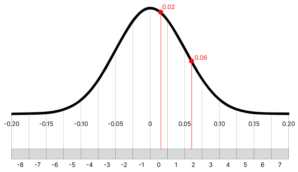
For example, the minimum/maximum of the distribution is [-0.2, 0.2]. This means that -0.2 will be converted to -8, and 0.2 to 7. Each number in the distribution will have a quantized equivalent in the interval (ex. the first number 0.02436554 will be quantized to -1).
array([[-1, -3, -1, ...,  1, -2, -2],
       [-6, -1, -2, ..., -2, -2, -3],
       [ 0, -2, -4, ..., -1,  1, -2],
       ...,
       [ 3,  0, -5, ..., -5,  7,  0],
       [-4, -5,  3, ..., -2, -2, -2],
       [-1,  0, -2, ..., -1,  1, -3]], dtype=int4)
1-bit quantization
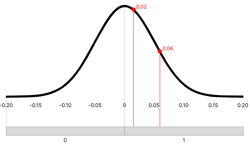
The same principle applies to binary quantization but is much simpler. The rule is the following: each number of the distribution < 0 becomes 0, and each number > 0 becomes 1.
Not all embeddings are built the same
The principal issue with current quantization techniques is that they live on the assumption that all our values are based on a single distribution. That is why, when we use thresholds to define intervals (ex. minimum and maximum), we only use a single set derived from the totality of our data (which is modeled on a single distribution).

In an experiment, I have encoded 40.000 game descriptions into vectors. By looking at the data distributions of each feature, we can see that despite the efforts, there is no feature which is perfectly normalized: its mean could deviate from the target 0.
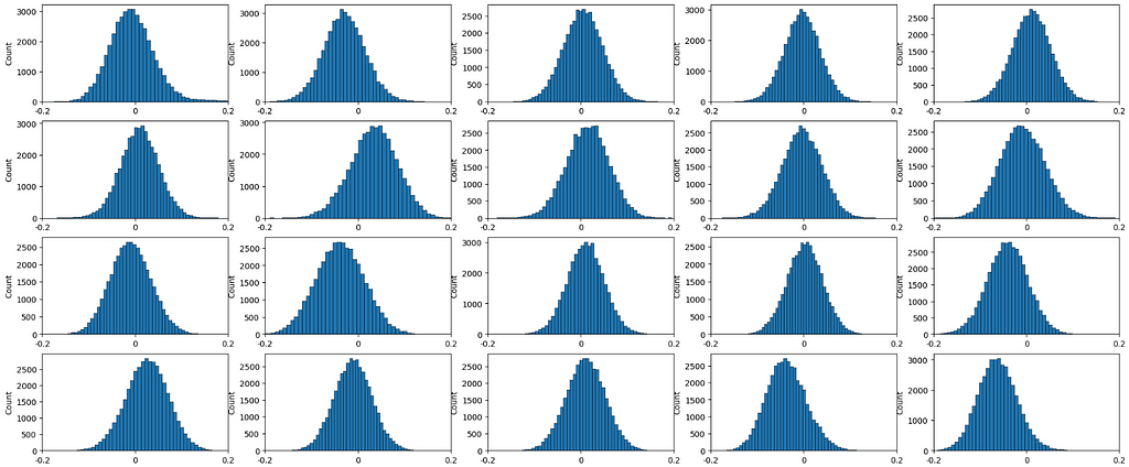
In a few words, each feature can be modeled with a dedicated distribution. Because the data does not follow a single giant distribution, we can leverage the many ways this is organized by applying a quantization at the feature level. In addition, embeddings tend to encode each feature using similar values (otherwise, the mean will constantly be 0), which means there is a minimal chance of drift when encoding additional data.
To better explain the math, let us define two sets of values:
S = all the individual samples from the encoded dataset (41936 * 384)
Fₙ = all the individual samples from the encoded dataset belonging to a single feature (41936 * 1)
Feature 29: The Ugly Duckling
In our sample dataset, each vector counts 384 features. However, by exploring the data one feature at a time, we can notice that some are not perfectly normalized but substantially skewed. Let us take F₂₉ as an example: the following plot shows the distribution of F₂₉ (41936) across our entire encoded dataset.

As we can see from the plot, its distribution mean is around -0.07, and its edges are (-0.2, 0.05). I am confident, knowing how encoders behave, that no matter the amount of extra data we are going to feed the model, F₂₉ will always remain an Ugly Duckling, with its distribution untouched. The distribution only counts a few positive values.
Regular Quantization
Now, let us apply binary quantization to the book, but only to F₂₉. I am choosing a binary approach because most of the information is lost, meaning there can be room for improvement using a different approach.
To quantize values in a binary fashion we need to pick a single value that will work as a threshold when converting values to either 0 or 1. The easiest way is to pick 0 (~ the distribution mean of S). When working on the values of F₂₉, because most of them are negative, the majority will be quantized to 0, and only a few will be quantized to 1.
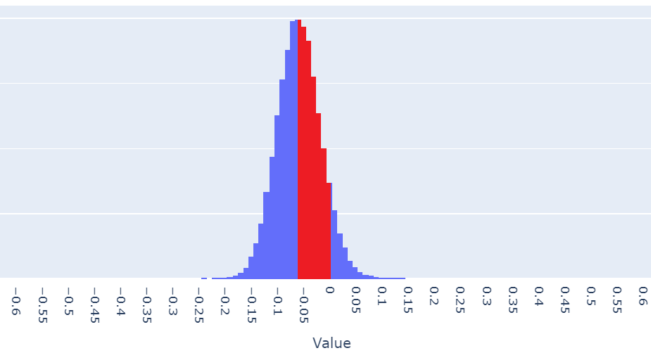
Let us explore the data further: 94% of the F₂₉ have been converted to 0, while our target in a perfectly normalized distribution is 50%. This means that 44% of F₂₉ (red area of the density distribution) has not been properly quantized.
# we count the number of 0 over the total number of values
>>> 1-quantized_regular[:, 29].sum()/sample_vectors[:, 29].size
0.9424122472338802
ft-Quantization
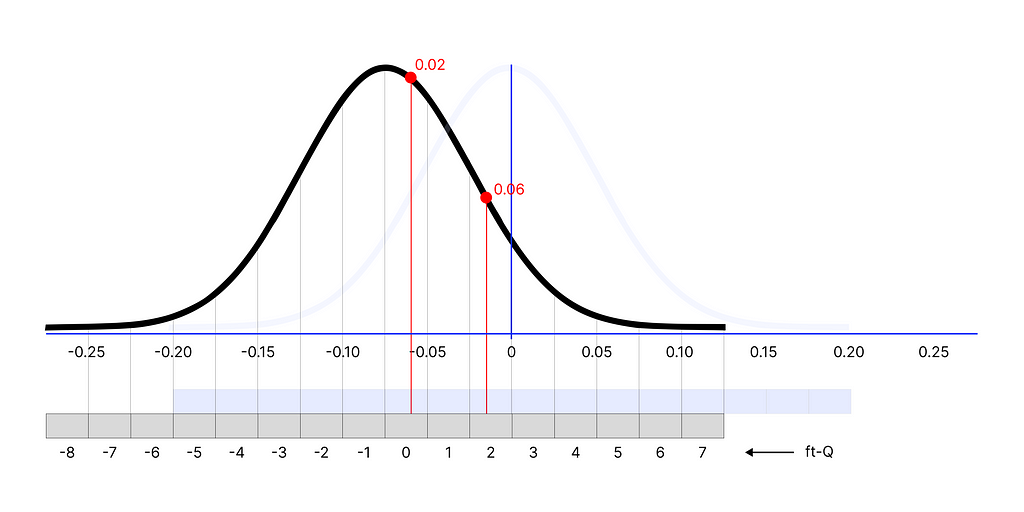
What if, instead of using 0 as a threshold (extracted from S) we were to use the F₂₉ distribution as a benchmark? Looking at F₂₉ distribution again, instead of 0, we would be using its mean ~ -0.07 and its extremes as the minimum/maximum of the interval ~ [-0.25, 0.15]. In simple words, ft-Q shifts the position of the reference quantization interval to better fit the real distribution of the data.
***Through the following article I am trying to introduce a new algorithm that, to the extent of my knowledge, I have been unable to find elsewhere. Note that the algorithm is different from FQ (feature quantization) that is used for training neural networks, this is algorithm is supposed to be used post-training.
I am open to criticism and welcome any feedback.
After applying binary quantization to F₂₉, because the threshold has been updated, we can see how half the times the data will be quantized to 0, and the other half to 1, resulting in a more realistic representation of the data. By comparing the quantization results, ft-Q has converted 47% of the F₂₉ into 0, resulting in only 3% of values not being properly quantized.
# we count the number of 0 over the total number of values
>>> 1-quantized_tfQ[:, 29].sum()/sample_vectors[:, 29].size
0.46809423884013734
To summarize, ft-Q (or ft-Quantization) encodes each feature individually, minimizing errors that can occur from non-normalized distributions.
When to use ft-Quantization
Realistically, no embedding is perfectly normalized, and there is a variance (despite it being minimal) across the feature distribution. However, now that we have identified the misplaced values, we can adjust them using
ft-Q.
Can ft-Q be applied to regular embeddings?
When ft-Q is applied to regular embeddings we are not looking at a substantial enhancement.
>>> err_regular = .5-quantized_regular.sum()/sample_vectors.size
>>> err_ftQ = .5-quantized_tfQ.sum()/sample_vectors.size
>>> err_total = abs(err_regular)-abs(err_ftQ)
>>> err_total
0.012901293538566672
In the case of all-MiniLM-L6-v2 we have reached a 1.2% improvement (not remarkable, but still an upgrade).
Where ft-Q shines: processed embeddings
However, embeddings are not always used in their normalized form. Sometimes, there are use cases where encoding requires the embedding to be processed (ex. in the case of covariate encoding). We can use the following theoretical diagram as a way to understand in which cases ft-Q can be better utilized:
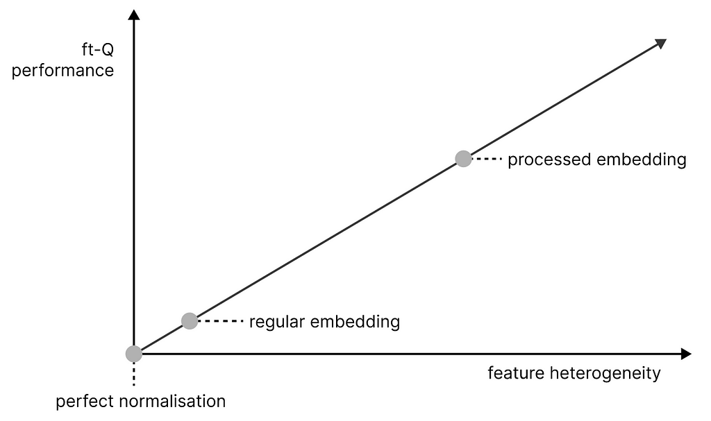
The vectors that are the result of an extra processing step are not necessarily normalized: we could normalize them again and only then apply quantization, but we can cast two birds with one stone by using ft-Q as a single operation (in addition to its small improvement even after a non-perfect normalization).
Conclusion
In conclusion, this article attempts to propose a more granular approach to quantization. Originally, the reason for developing this algorithm was to solve performance issues of processed embeddings, but after proper experimentation, it has proved useful even in a regular scenario.
After the popularization of LLM and more complex vector databases, memory management and performance improvements are becoming increasingly relevant in the space of information retrieval, hence it is our responsibility to familiarize ourselves with them and propose new and better solutions.
Time will tell if new and smarter data compression approaches will join the scene. For now, you can make the best use of this algorithm.
Introducing ft-Q: Improving Vector Compression with Feature-Level Quantization was originally published in Towards Data Science on Medium, where people are continuing the conversation by highlighting and responding to this story.
QuantizationPushing quantization to its limits by performing it at the feature level with ft-Quantization (ft-Q)***To understand this article, knowledge of embeddings and basic quantization is required. The implementation of this algorithm has been released on GitHub and is fully open-source.Since the dawn of LLMs, quantization has become one of the most popular memory-saving techniques for production-ready applications. Not long after, it has been popularized across vector databases, which have started using the same technology for compressing not only models but also vectors for retrieval purposes.In this article, I will showcase the limitations of the current quantization algorithms and propose a new quantization approach (ft-Q) to address them.What is Quantization and how does it work?Quantization is a memory-saving algorithm that lets us store numbers (both in-memory and in-disk) using a lower amount of bits. By default, when we store any number in memory, we use float32: this means that this number is stored using a combination of 32-bits (binary elements).For example, the integer 40 is stored as follows in a 32-bit object:storing the number 40 in a 32-bit object, image by AuthorHowever, we could decide to store the same number using fewer bits (cutting by half the memory usage), with a 16-bit object:storing the number 40 in a 16-bit object, image by AuthorBy quantization, we mean to store data using a lower number of bits (ex. 32 -> 16, or 32 -> 4), this is also known as casting. If we were to store 1GB of numbers (by default stored as 32-bit objects), if we decided to store them using 16-bit objects (hence, applying a quantization), the size of our data would be halved, resulting in 0.5GB.Is there a catch to quantization?Saving this amount of storage looks incredible (as you understood, we could keep cutting until we reach the minimum amount of bits: 1-bit, also known as binary quantization. Our database size will be reduced by 32 times, from 1GB to 31.25MB!), but as you might have already understood, there is a catch.Any number can be stored up to the limits allowed by all the possible combinations of bits. With a 32-bit quantization, you can store a maximum of 2³² numbers. There are so many possible combinations that we decided to include decimals when using 32-bits. For example, if we were to add a decimal to our initial number and store 40.12 in 32-bits, it would be using this combination of 1 and 0:01000010 00100000 01111010 11100001We have understood that with a 32-bit storage (given its large combination of possible values) we can pretty much encode each number, including its decimal points (to clarify, if you are new to quantization, the real number and decimal are not separated, 40.12 is converted as a whole into a combination of 32 binary numbers).If we keep diminishing the number of bits, all the possible combinations diminish exponentially. For example, 4-bit storage has a limit of 2⁴ combinations: we can only store 16 numbers (this does not leave much room to store decimals). With 1-bit storage, we can only store a single number, either a 1 or a 0.To put this into context, storing our initials 32-bit numbers into binary code would force us to convert all our numbers, such as 40.12 into either 0 or 1. In this scenario, this compression does not look very good.How to make the best out of QuantizationWe have seen how quantization results in an information loss. So, how can we make use of it, after all? When you look at the quantization of a single number (40.12 converted into 1), it seems there is no value that can derive from such an extreme level of quantization, there is simply too much loss.However, when we apply this technique to a set of data such as vectors, the information loss is not as drastic as when applied to a single number. Vector search is a perfect example of where to apply quantization in a useful manner.When we use an encoder, such as all-MiniLM-L6-v2, we store each sample (which was originally in the form of raw text) as a vector: a sequence of 384 numbers. The storage of millions of similar sequences, as you might have understood, is prohibitive, and we can use quantization to substantially diminish the size of the original vectors by a huge margin.Perhaps, quantizing our vectors from 32-bit to 16-bit is not this big of a loss. But how about 4-bit or even binary quantization? Because our sets are relatively large (384 numbers each), this considerable complexity lets us reach a higher level of compression without resulting in excessive retrieval loss.4-bit quantizationThe way we execute quantization is by looking at the data distribution of our flattened vector and choosing to map an equivalent interval with a lower number of bits. My favorite example is 4-bit quantization. With this degree of complexity, we can store 2⁴ = 16 numbers. But, as explained, all the numbers in our vectors are complex, each with several decimal points:array([ 2.43655406e-02, -4.33481708e-02, -1.89688837e-03, -3.76498550e-02, -8.96364748e-02, 2.96154656e-02, -5.79943173e-02, 1.87652372e-02, 1.87771711e-02, 6.30387887e-02, -3.23972516e-02, -1.46128759e-02, -3.39277312e-02, -7.04369228e-03, 3.87261175e-02, -5.02494797e-02, … -1.03239892e-02, 1.83096472e-02, -1.86534156e-03, 1.44851031e-02, -6.21072948e-02, -4.46912572e-02, -1.57684386e-02, 8.28376040e-02, -4.58770394e-02, 1.04658678e-01, 5.53084277e-02, -2.51113791e-02, 4.72703762e-02, -2.41811387e-03, -9.09169838e-02, 1.15215247e-02], dtype=float32)What we can do is map each of our numbers in the distribution into an interval that spans between [-8, 7] (16 possible numbers). To define the extreme of the interval, we can use the minimum and maximum values of the distribution we are quantizing.4-bit quantization: the grey area is an interval of integers between [-8, 7], don’t confuse it with bits. Any number of this interval will be later converted into a 4-bit object, image by AuthorFor example, the minimum/maximum of the distribution is [-0.2, 0.2]. This means that -0.2 will be converted to -8, and 0.2 to 7. Each number in the distribution will have a quantized equivalent in the interval (ex. the first number 0.02436554 will be quantized to -1).array([[-1, -3, -1, …, 1, -2, -2], [-6, -1, -2, …, -2, -2, -3], [ 0, -2, -4, …, -1, 1, -2], …, [ 3, 0, -5, …, -5, 7, 0], [-4, -5, 3, …, -2, -2, -2], [-1, 0, -2, …, -1, 1, -3]], dtype=int4)1-bit quantizationThe same principle applies to binary quantization but is much simpler. The rule is the following: each number of the distribution < 0 becomes 0, and each number > 0 becomes 1.1-bit quantization, image by AuthorNot all embeddings are built the sameThe principal issue with current quantization techniques is that they live on the assumption that all our values are based on a single distribution. That is why, when we use thresholds to define intervals (ex. minimum and maximum), we only use a single set derived from the totality of our data (which is modeled on a single distribution).distribution of all individual samples from a flattened encoded dataset, image by AuthorIn an experiment, I have encoded 40.000 game descriptions into vectors. By looking at the data distributions of each feature, we can see that despite the efforts, there is no feature which is perfectly normalized: its mean could deviate from the target 0.distributions of 20 random features of the encoded dataset, image by AuthorIn a few words, each feature can be modeled with a dedicated distribution. Because the data does not follow a single giant distribution, we can leverage the many ways this is organized by applying a quantization at the feature level. In addition, embeddings tend to encode each feature using similar values (otherwise, the mean will constantly be 0), which means there is a minimal chance of drift when encoding additional data.To better explain the math, let us define two sets of values:S = all the individual samples from the encoded dataset (41936 * 384)Fₙ = all the individual samples from the encoded dataset belonging to a single feature (41936 * 1)Feature 29: The Ugly DucklingIn our sample dataset, each vector counts 384 features. However, by exploring the data one feature at a time, we can notice that some are not perfectly normalized but substantially skewed. Let us take F₂₉ as an example: the following plot shows the distribution of F₂₉ (41936) across our entire encoded dataset.F₂₉ distribution, image by AuthorAs we can see from the plot, its distribution mean is around -0.07, and its edges are (-0.2, 0.05). I am confident, knowing how encoders behave, that no matter the amount of extra data we are going to feed the model, F₂₉ will always remain an Ugly Duckling, with its distribution untouched. The distribution only counts a few positive values.Regular QuantizationNow, let us apply binary quantization to the book, but only to F₂₉. I am choosing a binary approach because most of the information is lost, meaning there can be room for improvement using a different approach.To quantize values in a binary fashion we need to pick a single value that will work as a threshold when converting values to either 0 or 1. The easiest way is to pick 0 (~ the distribution mean of S). When working on the values of F₂₉, because most of them are negative, the majority will be quantized to 0, and only a few will be quantized to 1.samples whose quantized value should be 1, but quantized as 0: 44% of F₂₉, image by AuthorLet us explore the data further: 94% of the F₂₉ have been converted to 0, while our target in a perfectly normalized distribution is 50%. This means that 44% of F₂₉ (red area of the density distribution) has not been properly quantized.# we count the number of 0 over the total number of values>>> 1-quantized_regular[:, 29].sum()/sample_vectors[:, 29].size0.9424122472338802 ft-QuantizationWhat if, instead of using 0 as a threshold (extracted from S) we were to use the F₂₉ distribution as a benchmark? Looking at F₂₉ distribution again, instead of 0, we would be using its mean ~ -0.07 and its extremes as the minimum/maximum of the interval ~ [-0.25, 0.15]. In simple words, ft-Q shifts the position of the reference quantization interval to better fit the real distribution of the data.visualization of ft-Q, the interval is adapted to the feature distribution, image by Author***Through the following article I am trying to introduce a new algorithm that, to the extent of my knowledge, I have been unable to find elsewhere. Note that the algorithm is different from FQ (feature quantization) that is used for training neural networks, this is algorithm is supposed to be used post-training.I am open to criticism and welcome any feedback.After applying binary quantization to F₂₉, because the threshold has been updated, we can see how half the times the data will be quantized to 0, and the other half to 1, resulting in a more realistic representation of the data. By comparing the quantization results, ft-Q has converted 47% of the F₂₉ into 0, resulting in only 3% of values not being properly quantized.# we count the number of 0 over the total number of values>>> 1-quantized_tfQ[:, 29].sum()/sample_vectors[:, 29].size0.46809423884013734To summarize, ft-Q (or ft-Quantization) encodes each feature individually, minimizing errors that can occur from non-normalized distributions.When to use ft-QuantizationRealistically, no embedding is perfectly normalized, and there is a variance (despite it being minimal) across the feature distribution. However, now that we have identified the misplaced values, we can adjust them using ft-Q.Can ft-Q be applied to regular embeddings?When ft-Q is applied to regular embeddings we are not looking at a substantial enhancement.>>> err_regular = .5-quantized_regular.sum()/sample_vectors.size>>> err_ftQ = .5-quantized_tfQ.sum()/sample_vectors.size>>> err_total = abs(err_regular)-abs(err_ftQ)>>> err_total0.012901293538566672In the case of all-MiniLM-L6-v2 we have reached a 1.2% improvement (not remarkable, but still an upgrade).Where ft-Q shines: processed embeddingsHowever, embeddings are not always used in their normalized form. Sometimes, there are use cases where encoding requires the embedding to be processed (ex. in the case of covariate encoding). We can use the following theoretical diagram as a way to understand in which cases ft-Q can be better utilized:the more the feature skew from a perfect normalisation, the more ft-Q is effective, image by AuthorThe vectors that are the result of an extra processing step are not necessarily normalized: we could normalize them again and only then apply quantization, but we can cast two birds with one stone by using ft-Q as a single operation (in addition to its small improvement even after a non-perfect normalization).ConclusionIn conclusion, this article attempts to propose a more granular approach to quantization. Originally, the reason for developing this algorithm was to solve performance issues of processed embeddings, but after proper experimentation, it has proved useful even in a regular scenario.After the popularization of LLM and more complex vector databases, memory management and performance improvements are becoming increasingly relevant in the space of information retrieval, hence it is our responsibility to familiarize ourselves with them and propose new and better solutions.Time will tell if new and smarter data compression approaches will join the scene. For now, you can make the best use of this algorithm.Introducing ft-Q: Improving Vector Compression with Feature-Level Quantization was originally published in Towards Data Science on Medium, where people are continuing the conversation by highlighting and responding to this story. quantization, thoughts-and-theory, llm, vector-database, vector-embeddings Towards Data Science – MediumRead More

 Add to favorites


0 Comments