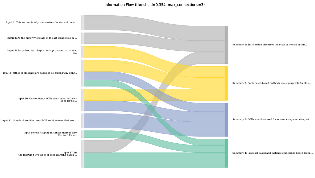
A fast and low-resource method using similarity-based attribution

TL;DR
- Explaining LLMs is very slow and resource-intensive.
- This article proposes a task-specific explanation technique or RAG Q&A and Summarization.
- The approach is model agnostic and is similarity-based.
- The approach is low-resource and low-latency, so can run almost everywhere.
- I provided the code on Github, using the Huggingface Transformers ecosystem.
Motivation
There are a lot of good reasons to get explanations for your model outputs. For example, they could help you find problems with your model, or they just could be a way to provide more transparency to the user, thereby facilitating user trust. This is why, for models like XGBoost, I have regularly applied methods like SHAP to get more insights into my model’s behavior.
Now, with myself more and more dealing with LLM-based ML systems, I wanted to explore ways of explaining LLM models the same way I did with more traditional ML approaches. However, I quickly found myself being stuck because:
- SHAP does offer examples for text-based models, but for me, they failed with newer models, as SHAP did not support the embedding layers.
- Captum also offers a tutorial for LLM attribution; however, both presented methods also had their very specific drawbacks. Concretely, the perturbation-based method was simply too slow, while the gradient-based method was letting my GPU memory explode and ultimately failed.
After playing with quantization and even spinning up GPU cloud instances with still limited success I had enough I took a step back.
A Similarity-based Approach
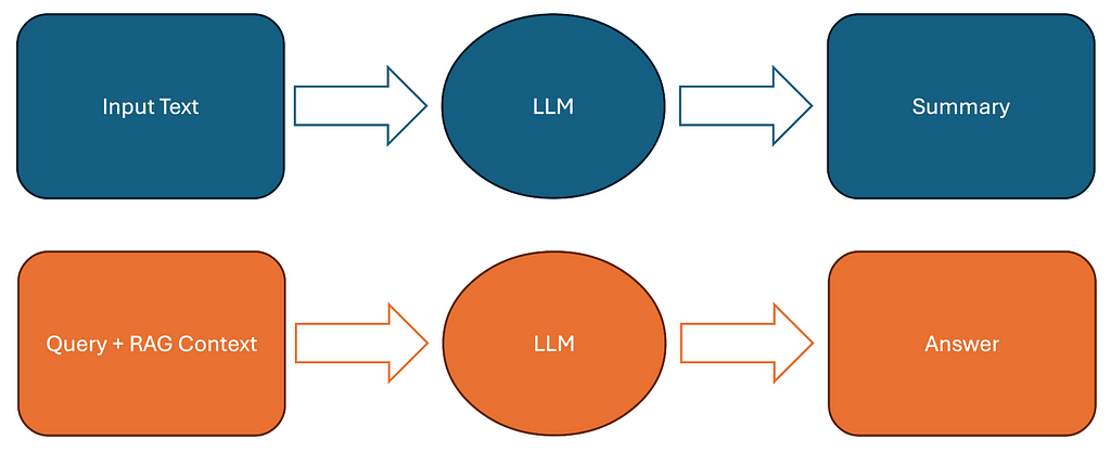
For understanding the approach, let’s first briefly define what we want to achieve. Concretely, we want to identify and highlight sections in our input text (e.g. long text document or RAG context) that are highly relevant to our model output (e.g., a summary or RAG answer).

In case of summarization, our method would have to highlight parts of the original input text that are highly reflected in the summary. In case of a RAG system, our approach would have to highlight document chunks from the RAG context that are showing up in the answer.
Since directly explaining the LLM itself has proven intractable for me, I instead propose to model the relation between model inputs and outputs via a separate text similarity model. Concretely, I implemented the following simple but effective approach:
- I split the model inputs and outputs into sentences.
- I calculate pairwise similarities between all sentences.
- I then normalize the similarity scores using Softmax
- After that, I visualize the similarities between input and output sentences in a nice plot
In code, this is implemented as shown below. For running the code you need the Huggingface Transformers, Sentence Transformers, and NLTK libraries.
Please, also check out this Github Repository for the full code accompanying this blog post.
from sentence_transformers import SentenceTransformer
from nltk.tokenize import sent_tokenize
import numpy as np

# Original text truncated for brevity ...
text = """This section briefly summarizes the state of the art in the area of semantic segmentation and semantic instance segmentation. As the majority of state-of-the-art techniques in this area are deep learning approaches we will focus on this area. Early deep learning-based approaches that aim at assigning semantic classes to the pixels of an image are based on patch classification. Here the image is decomposed into superpixels in a preprocessing step e.g. by applying the SLIC algorithm [1].

Other approaches are based on so-called Fully Convolutional Neural Networks (FCNs). Here not an image patch but the whole image are taken as input and the output is a two-dimensional feature map that assigns class probabilities to each pixel. Conceptually FCNs are similar to CNNs used for classification but the fully connected layers are usually replaced by transposed convolutions which have learnable parameters and can learn to upsample the extracted features to the final pixel-wise classification result. ..."""

# Define a concise summary that captures the key points
summary = "Semantic segmentation has evolved from early patch-based classification approaches using superpixels to more advanced Fully Convolutional Networks (FCNs) that process entire images and output pixel-wise classifications."

# Load the embedding model
model = SentenceTransformer('BAAI/bge-small-en')

# Split texts into sentences
input_sentences = sent_tokenize(text)
summary_sentences = sent_tokenize(summary)

# Calculate embeddings for all sentences
input_embeddings = model.encode(input_sentences)
summary_embeddings = model.encode(summary_sentences)

# Calculate similarity matrix using cosine similarity
similarity_matrix = np.zeros((len(summary_sentences), len(input_sentences)))
for i, sum_emb in enumerate(summary_embeddings):
    for j, inp_emb in enumerate(input_embeddings):
        similarity = np.dot(sum_emb, inp_emb) / (np.linalg.norm(sum_emb) * np.linalg.norm(inp_emb))
        similarity_matrix[i, j] = similarity

# Calculate final attribution scores (mean aggregation)
final_scores = np.mean(similarity_matrix, axis=0)

# Create and print attribution dictionary
attributions = {
    sentence: float(score)
    for sentence, score in zip(input_sentences, final_scores)
}

print("nInput sentences and their attribution scores:")
for sentence, score in attributions.items():
    print(f"nScore {score:.3f}: {sentence}")
So, as you can see, so far, that is pretty simple. Obviously, we don’t explain the model itself. However, we might be able to get a good sense of relations between input and output sentences for this specific type of tasks (summarization / RAG Q&A). But how does this actually perform and how to visualize the attribution results to make sense of the output?
Evaluation for RAG and Summarization
To visualize the outputs of this approach, I created two visualizations that are suitable for showing the feature attributions or connections between input and output of the LLM, respectively.
These visualizations were generated for a summary of the LLM input that goes as follows:
This section discusses the state of the art in semantic segmentation and instance segmentation, focusing on deep learning approaches. Early patch classification methods use superpixels, while more recent fully convolutional networks (FCNs) predict class probabilities for each pixel. FCNs are similar to CNNs but use transposed convolutions for upsampling. Standard architectures include U-Net and VGG-based FCNs, which are optimized for computational efficiency and feature size. For instance segmentation, proposal-based and instance embedding-based techniques are reviewed, including the use of proposals for instance segmentation and the concept of instance embeddings.
Visualizing the Feature Attributions
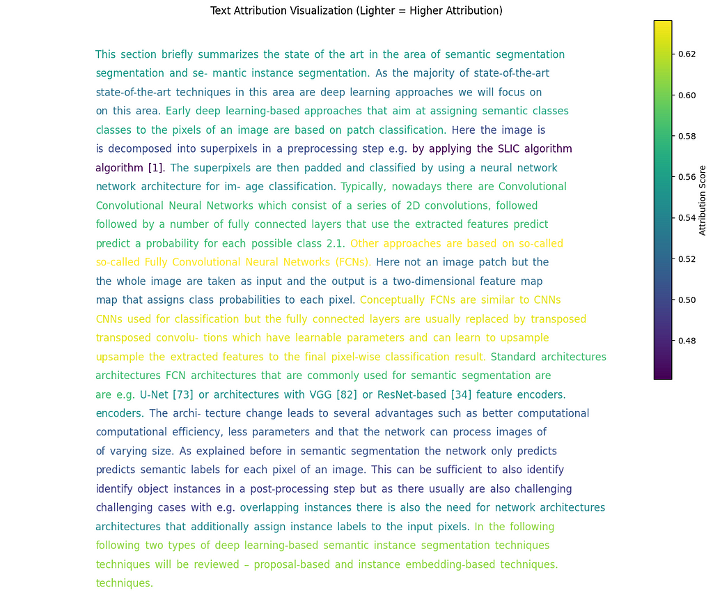
For visualizing the feature attributions, my choice was to simply stick to the original representation of the input data as close as possible.

Concretely, I simply plot the sentences, including their calculated attribution scores. Therefore, I map the attribution scores to the colors of the respective sentences.
In this case, this shows us some dominant patterns in the summarization and the source sentences that the information might be stemming from. Concretely, the dominance of mentions of FCNs as an architecture variant mentioned in the text, as well as the mention of proposal- and instance embedding-based instance segmentation methods, are clearly highlighted.
In general, this method turned out to work pretty well for easily capturing attributions on the input of a summarization task, as it is very close to the original representation and adds very low clutter to the data. I could imagine also providing such a visualization to the user of a RAG system on demand. Potentially, the outputs could also be further processed to threshold to certain especially relevant chunks; then, this could also be displayed to the user by default to highlight relevant sources.
Again, check out the Github Repository to get the visualization code
Visualizing the Information Flow
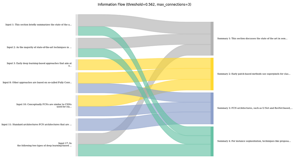
Another visualization technique focuses not on the feature attributions, but mostly on the flow of information between input text and summary.

Concretely, what I do here, is to first determine the major connections between input and output sentences based on the attribution scores. I then visualize those connections using a Sankey diagram. Here, the width of the flow connections is the strength of the connection, and the coloring is done based on the sentences in the summary for better traceability.
Here, it shows that the summary mostly follows the order of the text. However, there are few parts where the LLM might have combined information from the beginning and the end of the text, e.g., the summary mentions a focus on deep learning approaches in the first sentence. This is taken from the last sentence of the input text and is clearly shown in the flow chart.
In general, I found this to be useful, especially to get a sense on how much the LLM is aggregating information together from different parts of the input, rather than just copying or rephrasing certain parts. In my opinion, this can also be useful to estimate how much potential for error there is if an output is relying too much on the LLM for making connections between different bits of information.
Possible Extensions and Adaptations
In the code provided on Github I implemented certain extensions of the basic approach shown in the previous sections. Concretely I explored the following:
- Use of different aggregations, such as max, for the similarity score.
This can make sense as not necessarily the mean similarity to output sentences is relevant. Already one good hit could be relevant for out explanation. - Use of different window sizes, e.g., taking chunks of three sentences to compute similarities.
This again makes sense if suspecting that one sentence alone is not enough content to truly capture relatedness of two sentences so a larger context is created. - Use of cross-encoding-based models, such as rerankers.
This could be useful as rerankers are more rexplicitely modeling the relatedness of two input documents in one model, being way more sensitive to nuanced language in the two documents. See also my recent post on Towards Data Science.
As said, all this is demoed in the provided Code so make sure to check that out as well.
Conclusion
In general, I found it pretty challenging to find tutorials that truly demonstrate explainability techniques for non-toy scenarios in RAG and summarization. Especially techniques that are useful in “real-time” scenarios, and are thus providing low-latency seemed to be scarce. However, as shown in this post, simple solutions can already give quite nice results when it comes to showing relations between documents and answers in a RAG use case. I will definitely explore this further and see how I can probably use that in RAG production scenarios, as providing traceable outputs to the users has proven invaluable to me. If you are interested in the topic and want to get more content in this style, follow me here on Medium and on LinkedIn.
Explaining LLMs for RAG and Summarization was originally published in Towards Data Science on Medium, where people are continuing the conversation by highlighting and responding to this story.
A fast and low-resource method using similarity-based attributionInformation flow between an input document and its summary as computed by the proposed explainability method. (image created by author)TL;DRExplaining LLMs is very slow and resource-intensive.This article proposes a task-specific explanation technique or RAG Q&A and Summarization.The approach is model agnostic and is similarity-based.The approach is low-resource and low-latency, so can run almost everywhere.I provided the code on Github, using the Huggingface Transformers ecosystem.MotivationThere are a lot of good reasons to get explanations for your model outputs. For example, they could help you find problems with your model, or they just could be a way to provide more transparency to the user, thereby facilitating user trust. This is why, for models like XGBoost, I have regularly applied methods like SHAP to get more insights into my model’s behavior.Now, with myself more and more dealing with LLM-based ML systems, I wanted to explore ways of explaining LLM models the same way I did with more traditional ML approaches. However, I quickly found myself being stuck because:SHAP does offer examples for text-based models, but for me, they failed with newer models, as SHAP did not support the embedding layers.Captum also offers a tutorial for LLM attribution; however, both presented methods also had their very specific drawbacks. Concretely, the perturbation-based method was simply too slow, while the gradient-based method was letting my GPU memory explode and ultimately failed.After playing with quantization and even spinning up GPU cloud instances with still limited success I had enough I took a step back.A Similarity-based ApproachFor understanding the approach, let’s first briefly define what we want to achieve. Concretely, we want to identify and highlight sections in our input text (e.g. long text document or RAG context) that are highly relevant to our model output (e.g., a summary or RAG answer).Typical flow of tasks our explainability method is applicable to. (image created by author)In case of summarization, our method would have to highlight parts of the original input text that are highly reflected in the summary. In case of a RAG system, our approach would have to highlight document chunks from the RAG context that are showing up in the answer.Since directly explaining the LLM itself has proven intractable for me, I instead propose to model the relation between model inputs and outputs via a separate text similarity model. Concretely, I implemented the following simple but effective approach:I split the model inputs and outputs into sentences.I calculate pairwise similarities between all sentences.I then normalize the similarity scores using SoftmaxAfter that, I visualize the similarities between input and output sentences in a nice plotIn code, this is implemented as shown below. For running the code you need the Huggingface Transformers, Sentence Transformers, and NLTK libraries.Please, also check out this Github Repository for the full code accompanying this blog post.from sentence_transformers import SentenceTransformerfrom nltk.tokenize import sent_tokenizeimport numpy as np# Original text truncated for brevity …text = “””This section briefly summarizes the state of the art in the area of semantic segmentation and semantic instance segmentation. As the majority of state-of-the-art techniques in this area are deep learning approaches we will focus on this area. Early deep learning-based approaches that aim at assigning semantic classes to the pixels of an image are based on patch classification. Here the image is decomposed into superpixels in a preprocessing step e.g. by applying the SLIC algorithm [1].Other approaches are based on so-called Fully Convolutional Neural Networks (FCNs). Here not an image patch but the whole image are taken as input and the output is a two-dimensional feature map that assigns class probabilities to each pixel. Conceptually FCNs are similar to CNNs used for classification but the fully connected layers are usually replaced by transposed convolutions which have learnable parameters and can learn to upsample the extracted features to the final pixel-wise classification result. …”””# Define a concise summary that captures the key pointssummary = “Semantic segmentation has evolved from early patch-based classification approaches using superpixels to more advanced Fully Convolutional Networks (FCNs) that process entire images and output pixel-wise classifications.”# Load the embedding modelmodel = SentenceTransformer(‘BAAI/bge-small-en’)# Split texts into sentencesinput_sentences = sent_tokenize(text)summary_sentences = sent_tokenize(summary)# Calculate embeddings for all sentencesinput_embeddings = model.encode(input_sentences)summary_embeddings = model.encode(summary_sentences)# Calculate similarity matrix using cosine similaritysimilarity_matrix = np.zeros((len(summary_sentences), len(input_sentences)))for i, sum_emb in enumerate(summary_embeddings): for j, inp_emb in enumerate(input_embeddings): similarity = np.dot(sum_emb, inp_emb) / (np.linalg.norm(sum_emb) * np.linalg.norm(inp_emb)) similarity_matrix[i, j] = similarity# Calculate final attribution scores (mean aggregation)final_scores = np.mean(similarity_matrix, axis=0)# Create and print attribution dictionaryattributions = { sentence: float(score) for sentence, score in zip(input_sentences, final_scores)}print(“nInput sentences and their attribution scores:”)for sentence, score in attributions.items(): print(f”nScore {score:.3f}: {sentence}”)So, as you can see, so far, that is pretty simple. Obviously, we don’t explain the model itself. However, we might be able to get a good sense of relations between input and output sentences for this specific type of tasks (summarization / RAG Q&A). But how does this actually perform and how to visualize the attribution results to make sense of the output?Evaluation for RAG and SummarizationTo visualize the outputs of this approach, I created two visualizations that are suitable for showing the feature attributions or connections between input and output of the LLM, respectively.These visualizations were generated for a summary of the LLM input that goes as follows:This section discusses the state of the art in semantic segmentation and instance segmentation, focusing on deep learning approaches. Early patch classification methods use superpixels, while more recent fully convolutional networks (FCNs) predict class probabilities for each pixel. FCNs are similar to CNNs but use transposed convolutions for upsampling. Standard architectures include U-Net and VGG-based FCNs, which are optimized for computational efficiency and feature size. For instance segmentation, proposal-based and instance embedding-based techniques are reviewed, including the use of proposals for instance segmentation and the concept of instance embeddings.Visualizing the Feature AttributionsFor visualizing the feature attributions, my choice was to simply stick to the original representation of the input data as close as possible.Visualization of sentence-wise feature attribution scores based on color mapping. (image created by author)Concretely, I simply plot the sentences, including their calculated attribution scores. Therefore, I map the attribution scores to the colors of the respective sentences.In this case, this shows us some dominant patterns in the summarization and the source sentences that the information might be stemming from. Concretely, the dominance of mentions of FCNs as an architecture variant mentioned in the text, as well as the mention of proposal- and instance embedding-based instance segmentation methods, are clearly highlighted.In general, this method turned out to work pretty well for easily capturing attributions on the input of a summarization task, as it is very close to the original representation and adds very low clutter to the data. I could imagine also providing such a visualization to the user of a RAG system on demand. Potentially, the outputs could also be further processed to threshold to certain especially relevant chunks; then, this could also be displayed to the user by default to highlight relevant sources.Again, check out the Github Repository to get the visualization codeVisualizing the Information FlowAnother visualization technique focuses not on the feature attributions, but mostly on the flow of information between input text and summary.Visualization of the information flow between sentences in Input text and summary as Sankey diagram. (image created by author)Concretely, what I do here, is to first determine the major connections between input and output sentences based on the attribution scores. I then visualize those connections using a Sankey diagram. Here, the width of the flow connections is the strength of the connection, and the coloring is done based on the sentences in the summary for better traceability.Here, it shows that the summary mostly follows the order of the text. However, there are few parts where the LLM might have combined information from the beginning and the end of the text, e.g., the summary mentions a focus on deep learning approaches in the first sentence. This is taken from the last sentence of the input text and is clearly shown in the flow chart.In general, I found this to be useful, especially to get a sense on how much the LLM is aggregating information together from different parts of the input, rather than just copying or rephrasing certain parts. In my opinion, this can also be useful to estimate how much potential for error there is if an output is relying too much on the LLM for making connections between different bits of information.Possible Extensions and AdaptationsIn the code provided on Github I implemented certain extensions of the basic approach shown in the previous sections. Concretely I explored the following:Use of different aggregations, such as max, for the similarity score.This can make sense as not necessarily the mean similarity to output sentences is relevant. Already one good hit could be relevant for out explanation.Use of different window sizes, e.g., taking chunks of three sentences to compute similarities.This again makes sense if suspecting that one sentence alone is not enough content to truly capture relatedness of two sentences so a larger context is created.Use of cross-encoding-based models, such as rerankers.This could be useful as rerankers are more rexplicitely modeling the relatedness of two input documents in one model, being way more sensitive to nuanced language in the two documents. See also my recent post on Towards Data Science.As said, all this is demoed in the provided Code so make sure to check that out as well.ConclusionIn general, I found it pretty challenging to find tutorials that truly demonstrate explainability techniques for non-toy scenarios in RAG and summarization. Especially techniques that are useful in “real-time” scenarios, and are thus providing low-latency seemed to be scarce. However, as shown in this post, simple solutions can already give quite nice results when it comes to showing relations between documents and answers in a RAG use case. I will definitely explore this further and see how I can probably use that in RAG production scenarios, as providing traceable outputs to the users has proven invaluable to me. If you are interested in the topic and want to get more content in this style, follow me here on Medium and on LinkedIn.Explaining LLMs for RAG and Summarization was originally published in Towards Data Science on Medium, where people are continuing the conversation by highlighting and responding to this story. data-science, tips-and-tricks, explainable-ai, llm, machine-learning Towards Data Science – MediumRead More

 Add to favorites


0 Comments